The Normalizing Flow Network

The Normalizing Flow Network (NFN) is a normalizing-flow based regression model, great at modelling complex conditional densities. Look at our recent paper on noise regularization for conditional density estimation for some results of using the NFN on real-world and benchmark regression datasets.

Here I’ll explain the structure of the NFN and go through some of the math. Implementations can be found in our Open-Source Python package as well as in my repo.

Normalizing Flows

Let’s start with the density model, the final part of the NFN. We are using Normalizing Flows as a way to parametrize the distribution we are outputting. This expressive family can model characteristics of distributions like heteroscedasticityThis means that the variance of \(Y\) is not constant over \(X\). In this dataset for example, the variance of Y is higher for \(X\leq0\).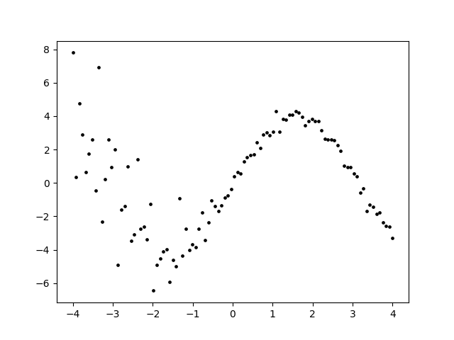 and fat tailsThe Cauchy distribution is one example of a fat-tailed distribution. Compared to a Gaussian, it has outliers that are far more likely (So far so that it’s mean cannot even be defined)..

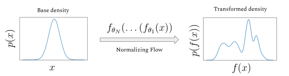
A Normalizing Flow turns a simple base distribution \(p(x)\) (e.g. a Uniform or Gaussian distribution) into a more complex distribution \(\hat{p}(y)\). This is done by applying an invertible, parametric function \(f(x)\) to samples \(x\) drawn from the base distribution, resulting in samples \(y\) from the transformed distribution.

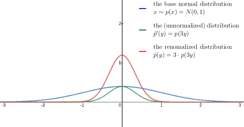
Let’s start with a simple example: Take a random variable \(X\) distributed according to a Normal distribution with zero mean and uniform variance. What is the distribution of, say \(Y = f(X) = \frac{1}{3} \cdot X\)? Since we divide every sample \(x \sim p(X)\) by 3 to get a sample \(y \sim \hat{p}(Y)\), we can expect the distribution of Y to be more narrow, with most samples being closer to the mean than in the base distribution.

Now how to we calculate the density of Y? A sample \(y \sim \hat{p}(Y)\) is generated by sampling \(x \sim p(X)\) and then transforming it to get \(f(x) = y\). For a given sample y, we can get the x that generated it by using the inverse transformation \(f^{-1}(y) = 3y = x\). We can then calculate the likelihood of this x: \(p(f^{-1}(y)) = p(x) = p(3y)\). Yet that is not equal to the likelihood of our sample y. Since the density has been compressed, samples in the neighbourhood of y will be more likely than they had been under the (more stretched out) standard normal distribution. This can be seen in the plot, the distribution \(p(3y)\) is degenerate and doesn’t integrate to 1. Therefore we need to normalize. This can be done by multiplying with the absolute derivative of the inverse of our function, \(|\frac{df^{-1}}{dy}| = |\frac{df}{dx}|^{-1}\).

This makes intuitive sense:

• \(\vert\frac{df}{dx}\vert \leq 1\): The function has a compressing effect. Samples closer together will be more likely so we need to scale up the transformed density.
• \(\vert\frac{df}{dx}\vert > 1\): The function expands the original density. Samples closer together will be less likely and we need to scale down to normalize.

For multivariate distributions, the absolute derivate of the inverse function becomes the absolute determinant of the jacobian of the inverse function: \(\mid\det \frac{\partial f^{-1}}{\partial \mathbf{y}}\mid\).While it’s a little harder to get an intuition for why that is the case, consider affine transformations in higher dimensions. They are easier to visualize than the general case since their Jacobian is just the transformation matrix. The determinant of a matrix is nothing but the amount of volume change resulting from the affine transformation defined by the matrix. For the 2-D case, check out this applet. Image the ‘M’ as a square. Then change the transformation matrix and see how the volume of the square is proportional to the determinant of the matrix. This leads us to the main formula of Normalizing Flows which tells us how to normalize a distribution transformed by \(f(\mathbf{x})\):

This equation can be derived using the change-of-variable theorem. \(f(\mathbf{x})\) has to be continuously differentiable and invertible. Many of such functions have been proposed. For the NFN we implemented three of them that we have found to be both expressive and fast to compute: affine, planar and radial flows.We picked those three because unlike some of the recent flows like MAF or Real NVP they work especially well for low-dimensional densities.

Affine Flows

The example I used in the beginning of this post is an instance of the Affine Normalizing Flow:

They are the simplest Normalizing Flow and can be used to shift and scale distributions.They are not able to split a distribution into two modes though. To model multimodal distributions, we will combine them with other Normalizing Flows. Here we use an affine flow to transform a standard normal distribution:

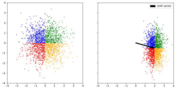
The initial 2-D Gaussian is shifted and compressed, yet stays Gaussian. \(\mathbf{a}\) controls the scaling of the distribution and \(\mathbf{b}\) is the shift vector.

Planar Flows

Planar Flows compress and expand densities around a hyperplane:

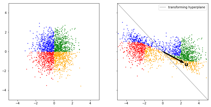
The Gaussian base distribution is split into two halfs in this example. \(b\) and \(\mathbf{w}\) define the hyperplane whereas \(\mathbf{u}\) specifies the direction and strength of the expansion.Side note: While equation (3) is invertible using the right constraints, no closed form inverse is know. Therefore in practice the inverse can only be approximated.

Radial Flows

Radial flows compress and expand around a reference point:

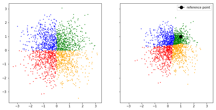
\(\gamma\) is the reference point, \(\alpha, \beta\) specify how strongly to compress / expand.

Both planar and radial flows are only invertible functions if their parameters are correctly constrained. How to constrain each flow and how to calculate the inverse log determinant of the Jacobian is explained in the documentation for my code and in Rezende and Mohamed (2015).

Applying one Normalizing Flow to a distribution results in another distribution. Therefore we can stack multiple flows to get even more expressive transformed distributionsTwo consecutive planar flows transforming an initially Gaussian distribution: .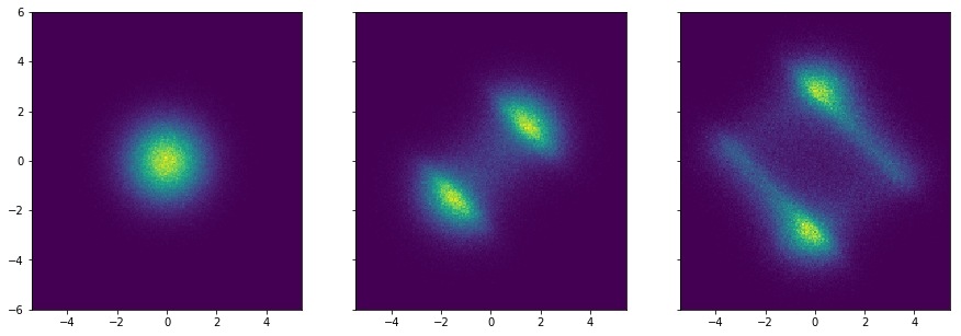

The Normalizing Flow Network

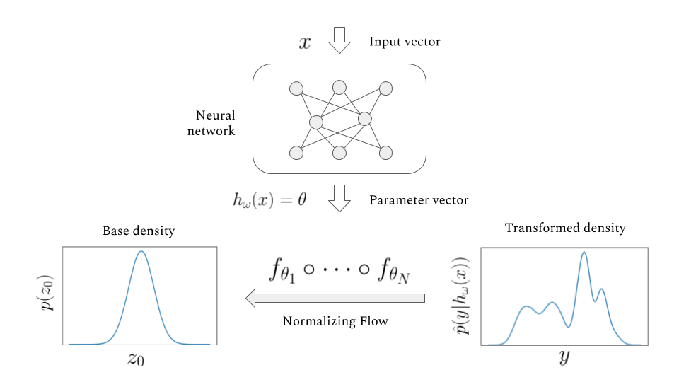
Now let’s combine the Normalizing Flows with a neural network that allows us to model conditional distributions. This concept is similar to a Mixture Density Network.For the MDN the density model is a Mixture of Gaussians, for the NFN it’s a Normalizing Flow. The NFN is used to predict the conditional distribution \(p(y|x)\).This is a generalization of regression / classification. In a regular regression task for example, one predicts y given x as \(\mathbb{E}(y|x)\). We generalize this by predicting a full distribution instead of just a point estimate. Say \(x\) is a job title and we’re trying to predict \(y\), the salary associated with it.For example for p(wage | job=’lawyer’), this conditional distribution is strongly bimodal as you can see here. Some lawyers are much better off than others. The NFN now works as follows:

1. A neural net takes x as it’s input and outputs the parameters of a stack of Normalizing Flows, e.g. two planar flows and one affine flow (The exact setup of the flow is a hyperparameter of the NFN).
2. The Normalizing Flows now define a transformation of a base Gaussian distribution into a more complex distribution, the conditional \(p(y\vert x)\).
3. The model is then trained to minimize the negative log likelihood of the data:

As a small detail, the Normalizing Flows are actually inverted in the NFN and point from the transformed distribution to the base distribution. This is mainly done to speed up the process, as the flows we use here we developed for posterior density estimation in variational inference by Rezende and Mohamed (2015). In their original form they are fast at sampling and slow at likelihood computation. For CDE we need the opposite.

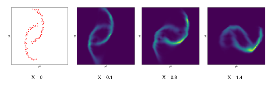
The NFN fitted on a conditional version of the two moons dataset where \(X\) determines the rotation of \(Y\) around the origin:

Conclusion

Normalizing flows serve as a powerful, novel way of parametrizing distributions. In the tests in our paper we compared the NFN against the Mixture Density Network and the Kernel Mixture Network, among others. The NFN shows favourable performance on datasets that are strongly non-Gaussian, e.g. datasets that exhibit skewness and heavy tails.

You can try the NFN and other conditional density estimators on your own data using our Python package (TensorFlow 1.X) or my repo (TensorFlow 2.0).

Further Info

• For more on Normalizing Flows, I can recommend the blog posts by Eric Jang as well as Lilian Weng’s blog.
• Normalizing Flows, as well as Conditional Density Estimation and Variational Inference where the subject of my undergraduate thesis.