lleaves - Compiling Decision Trees for Fast Prediction using LLVM
September 2021
Gradient-boosted decision trees are a commonly used machine learning algorithm that performs well on real-world tabular datasets. There are many libraries available for training them, most commonly LightGBM and XGBoost. Sadly few of the popular libraries are optimized for fast prediction & deployment. As a remedy, I spent the last few months building lleaves, an open-source decision tree compiler and Python package.
It can be used as a drop-in replacement for LightGBM and speeds up inference by ≥10x. lleaves compiles decision trees via LLVM to generate optimized machine code. My goal is for lleaves to make state-of-the-art prediction speedups available to every Data Scientist. Check out the repo and install via pippip install lleaves or conda-forge!conda install -c conda-forge lleaves
Why use lleaves?
lleaves is fast, easy to use, and supports all standard features of LightGBM. To demonstrate, I’ll use a LightGBM model trained on the MTPL2 dataset. Compiling this model with lleaves is easy:
model = lleaves.Model(model_file="MTPL2/model.txt")
model.compile()
result = model.predict(df)
The runtime drops from 9.7s (LightGBM) to 0.4s (lleaves).If you’re using tree models interactively, this speedup makes for quite a stark difference. Here we’re predicting on large batches using multithreading. lleaves works similarly well for single-threaded prediction on small batches.
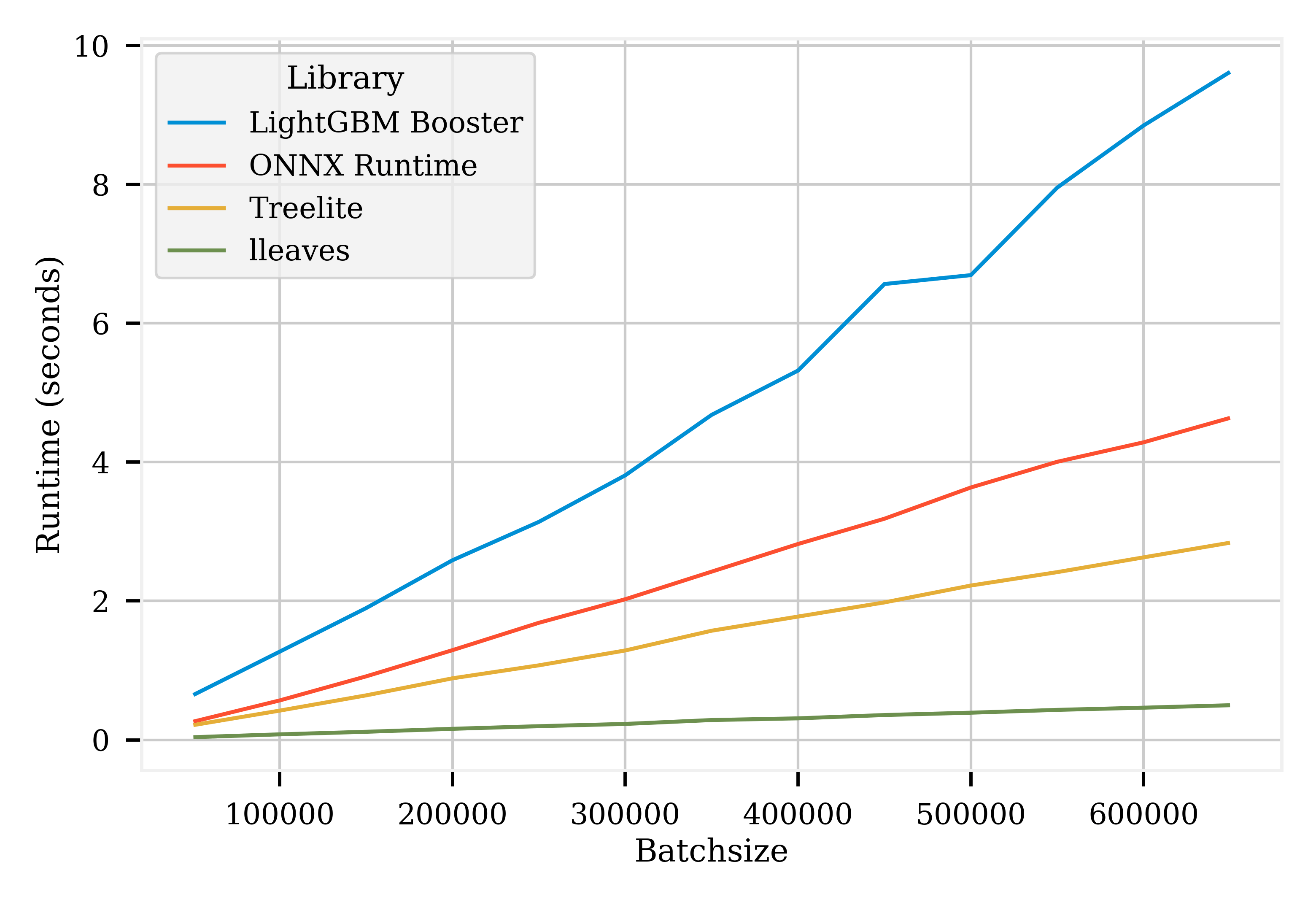
The benchmarks compare lleaves to ONNX and treelite, two other libraries that compile decision trees for prediction on CPU.
How does lleaves work?This is a high-level overview over the compiler-architecture of lleaves, mainly targeted at Data Scientists. I’m working on a second post detailing the performance optimizations that went into the library. Follow me on Twitter to be notified when I publish it.
lleaves is a compiler, meaning it converts code from one language into another language.
More precisely: lleaves is a frontend to the LLVM compiler toolkit, turning the LightGBM’s model.txt into LLVM IR (I’ll soon explain what these words mean).
In the end, we need our trained model to be turned into assembly code that the CPU can understand.
The full compilation happens in 3 steps:
- LightGBM stores the trained model in a
model.txt-file on disk. - lleaves loads the
model.txtand converts it to LLVM IR. - LLVM converts the LLVM IR to native assembly.
lleaves relies heavily on LLVM to generate the assembly. LLVM is a “compiler toolkit” meaning it provides modules and parts to make building compilers easier. One of these parts is the LLVM Intermediate Representation (IR), a low-level programming language that looks similar to RISC assembly. The IR is not yet machine code, so it still needs to be converted before it can be executed by the CPU.
The architecture of lleaves is similar to many modern compilers like clang (C/C++), rustc (Rust) or numba (Python), albeit much less complicated.
Modern Compiler Architecture
A modern compiler consists of three phases, which look like this:
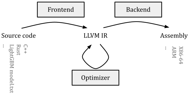
- The frontend transforms the source code into an architecture-independent intermediate representation (IR).
- The optimizer takes the generated IR and runs optimization passes over it. These passes output IR again but might remove redundant code or replace expensive operations with equal but faster ones.
- The optimized IR is passed to the compiler’s backend that turns the IR into assembly. Architecture-specific optimizations also take place during this step.
The LLVM toolkit specifies the LLVM IR and includes an optimizer as well as the backend. This means with LLVM, all that’s necessary for writing a new compiler is proving a frontend that converts source code into LLVM IR. Then LLVM’s optimizer and backend tune the IR and convert it to assembly.In reality, it’s slightly more complicated. For example, many compilers (like numba) include their own, more high-level IR to run language-specific optimizations more easily before ultimately lowering to LLVM IR.
Remember how I said lleaves is a frontend for LLVM?
That is because lleaves converts the model.txt outputted by LightGBM into LLVM IR.
Then lleaves passes the IR to LLVM’s optimizer and backend, which handles the final conversion to machine code (assembly).
Step 1: LightGBM ↦ Model.txt
To illustrate, we’ll follow a trained LightGBM model through every conversion step from model.txt to assembly.
As a running example, let’s look at this single decision tree that was trained with LightGBM:
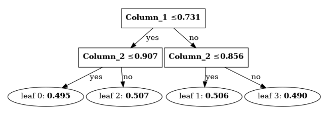
Each node in the tree compares the input value with its threshold. If the value is smaller than or equal to the threshold it takes the left path. Else, it goes right. Once we reach a leaf, the leaf’s value is returned.
LightGBM stores our example tree in a model.txt-file which looks something like this:For any real-world model there’d be 100+ trees here obviously, not just one.
Tree=0
num_leaves=4
threshold=0.731 0.907 0.856         # each node's threshold
split_feature=1 2 2                 # input feature to compare threshold with
left_child=1 -1 -2                  # for each node, index of left child
right_child=2 -3 -4                 # for each node, index of right child
leaf_value=0.495 0.507 0.506 0.490  # each leaf's return value
Step 2: Model.txt ↦ LLVM IR
lleaves loads this model.txt from disk, parses it, and converts the tree to LLVM IR:
define private double @tree_0(double %.1, double %.2, double %.3) {
node_0:
  %.5 = fcmp ule double %.2, 0x3FE768089A419B12   ; decimal = ~0.731
  br i1 %.5, label %node_1, label %node_2

node_1:                                           ; preds = %node_0
  %.7 = fcmp ule double %.3, 0x3FED06D4513F4FE5   ; decimal = ~0.907
  br i1 %.7, label %leaf_0, label %leaf_2

node_2:                                           ; preds = %node_0
  %.11 = fcmp ule double %.3, 0x3FEB60631F166F7A  ; decimal = ~0.856
  br i1 %.11, label %leaf_1, label %leaf_3

leaf_0:                                           ; preds = %node_1
  ret double 0x3FDFAFD3A55B8741                   ; decimal = ~0.495

leaf_2:                                           ; preds = %node_1
  ret double 0x3FE038704B651588                   ; decimal = ~0.507

leaf_1:                                           ; preds = %node_2
  ret double 0x3FE034DEA54DFC96                   ; decimal = ~0.506

leaf_3:                                           ; preds = %node_2
  ret double 0x3FDF62CFF241EA8B                   ; decimal = ~0.490
}
In the IR snippet, you can see how each node of the tree is processed.
The input data is passed via the function’s attributes (%.1, %.2, %.3).
The relevant attributes are float-compared (fcmp) with the threshold to check if the attribute is unsigned less-or-equal (ule) than the threshold.Every double has been converted into its hexadecimal representation.
Based on the result we jump/break (br) to the next node and finally return (ret) the result.
The model has now been converted into a low-level, standardized language. All that’s left to do is compile this to assembly.
Step 3: LLVM IR ↦ Assembly
After lleaves has converted the model to LLVM IR, LLVM runs optimization passes over it and tunes the code for the native CPU architecture. Then the final assembly code is generated. On an Intel CPU, the tree’s function now looks like this (truncated):Assembly is hard to read if you’re not used to it. Compare this to the LLVM IR above, which is much more easily understandable (and hence easier to generate, too!)
.LCPI0_0:
        .quad   0x3fe768089a419b12      ; double 0.731
.LCPI0_1:
        .quad   0x3feb60631f166f7a      ; double 0.856
.LCPI0_3:
        .quad   0x3fed06d4513f4fe5      ; double 0.907
.LCPI0_2:
        .quad   0x3fdf62cff241ea8b      ; double 0.490
        .quad   0x3fe034dea54dfc96      ; double 0.506
.LCPI0_4:
        .quad   0x3fe038704b651588      ; double 0.507
        .quad   0x3fdfafd3a55b8741      ; double 0.495
tree_0:                                 ; @tree_0
        xor     eax, eax
        ucomisd xmm1, qword ptr [rip + .LCPI0_0]
        ja      .LBB0_2
        ucomisd xmm2, qword ptr [rip + .LCPI0_3]
        setbe   al
        movsd   xmm0, qword ptr [8*rax + .LCPI0_4]
        ret
.LBB0_2:                                ; %node_2
        ucomisd xmm2, qword ptr [rip + .LCPI0_1]
        setbe   al
        movsd   xmm0, qword ptr [8*rax + .LCPI0_2]
        ret
To summarize the three compilation steps: The model is trained with LightGBM and saved to a model.txt.
lleaves then loads the model.txt and converts the model to architecture-agnostic LLVM IR.
The IR is passed to LLVM, optimized for the specific CPU architecture, and converted into assembly.
The final assembly can then be called from Python, passing in the data and returning the result.
Why can lleaves predict faster than LightGBM?
In LightGBM the relevant code looks like this:
inline int NumericalDecision(double fval, int node) const {
  if (fval <= threshold_[node]) {
    return left_child_[node];
  }
  return right_child_[node];
}
LightGBM doesn’t generate any code for its trained models.
Instead, the model.txt is loaded from disk into memory at runtime.
The tree is then executed node-by-node by calling NumericalDecision once for every node in the tree.
The decision-making function stays precisely the same for every tree and every node.
The model compilation inside lleaves works very differently by generating unique code for each decision node.
This compilation step allows for compile-time optimizations, removes the memory-access overhead, and unlocks modern CPU features, like branch prediction.
Conclusion
I regularly test lleaves on diverse models from inner-city parks (<100 trees) to black forests (>1000 trees) and see speedups anywhere from 10x to 30x. If you use LightGBM in your deployment, give lleaves a try! Installation instructions, docs & benchmarks can be found in the Github repository.
Notes
- Right now the code generation within lleaves is still somewhat simplistic. I’m working on making lleaves even faster through vectorizing parts of the generated code using algorithms like QuickScorer. So look out for future speedups!
- If you’re reading this and you know a lot about performance profiling, I’d love to talk to you! I have some questions about good benchmarking setups and need some seasoned advice 🙏.