Fast Multidimensional Matrix Multiplication on CPU from Scratch
August 2022
Numpy can multiply two 1024x1024 matrices on a 4-core Intel CPU in ~8ms. This is incredibly fast, considering this boils down to 18 FLOPs / core / cycle, with a cycle taking a third of a nanosecond. Numpy does this using a highly optimized BLAS implementation.BLAS is short for Basic Linear Algebra Subprograms. These are libraries providing fast implementations of eg Matrix multiplications or dot-products. They are sometimes tailored to one specific (family of) CPUs, like Intel’s MKL or Apple’s accelerate. However, non-Vendor specific implementations like OpenBLAS are also available. How hard is it to recreate performance that’s roughly similar using plain C++?
Calculating total FLOPs
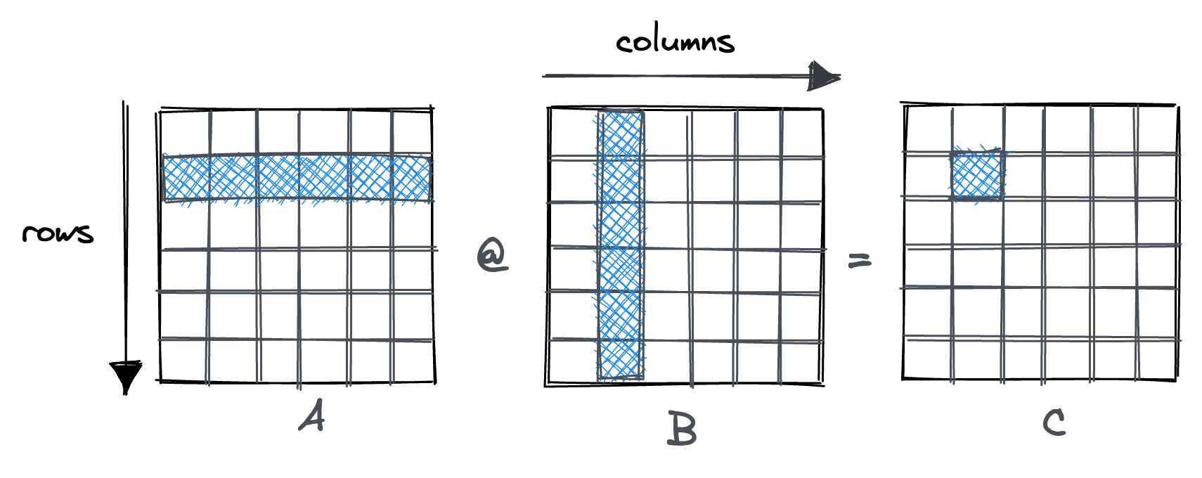
For simplicity, let’s assume both matrices are square. For each entry of our NxN result matrix, we have to perform a dot product between a row vector and a column vector, both of length N.
def MMM(A, B)
    C = np.zeros((A.n_rows, B.n_columns))
    for row in range(A.n_rows):
        for col in range(B.n_columns):
            for inner in range(A.n_inner):
                C[row, col] = C[row, col] + A[row, inner] * B[inner, col]
    return C
This results in N(=rows) * N(=columns) * N(=dot product) * 2(mul + add) = 2N³ FLOPs.
Running on a physical machine
In Numpy, the code for our example looks like this:
x = np.random.randn(1024, 1024).astype(np.float32)
y = np.random.randn(1024, 1024).astype(np.float32)
start = time.time_ns()
z = np.dot(x, y)
end = time.time_ns() - start
When I run this on my dedicated server, equipped with an Intel i7-6700 (a quad-core Haswell CPU) it takes 8ms.
- Total FLOPs: 2 Billion.
- Total memory (LOAD): 8MB using fp32.
- Total cycles: 8ms x 3.4GHz = 27 Million
That’s 18 FLOPS / core / cycle, or ~250GFLOP/s, on hardware released in 2015. That’s a lot!
How can a single core do 18 FLOPs in a cycle?
On my Haswell server, Numpy uses Intel’s MKL implementation of BLAS.
Particularly we care about how the SGEMM function is implemented, which is the function that is called for matrix multiplications.SGEMM is short for single-precision general matrix multiply. GEMM performs this computation: C = α*A*B + β*C. A,B,C are matrices and α,β are scalars.
Digging around the binary, there are multiple SGEMM implementations, each specific to one of Intel’s microarchitectures: eg sgemm_kernel_HASWELL, sgemm_kernel_SANDYBRIDGE, …
At runtime, the BLAS library will use the cpuid instruction to query the details of the processor and then call the suitable function.This will increase the size of the BLAS binary considerably since it’s carrying around GEMM implementations for many architectures, even though we ever only need one.
Looking closely at the relevant sgemm_kernel_HASWELL, the speed comes from using vectorizedA vectorized / SIMD instruction performs the same instruction on all entries of the vector input at once: FMAFMA stands for Fused Multiply Add. This means performing
 A = A + B*C, but using a single (fused) instruction. Sometimes this is also refered to as MAC (Multiply Accumulate). instructions, in my particular case the VFMADD instruction.
It operates on three 256bit long YMM registers, calculating (YMM1 * YMM2) + YMM3 and storing the result in YMM3.
That allows the CPU to perform 16 single-precision FLOPs in one instruction.
Checking Agner Fog’s instruction tables and uops.info, VFMADD has a throughputConfusingly, this is the reciprocal throughput, meaning the average number of clock cycles per instruction, for a series of independent instructions of the same kind in the same thread. of 0.5 cycles.
This means our theoretical upper limit should be 2 * VFMADD instructions per cycle, or 32 FLOPS / cycle.
At a latencyLatency here is the number of cycles between starting the instruction and having the result available to other instructions. of 5 cycles, this means we need to find 10 * 16 FLOPs that we can schedule independently, since the result of previous instructions is only available 5 cycles after they were started. This will be one consideration when writing optimized code: Grouping enough independent operations such that the CPU can schedule all of them at once, fully exploiting its instruction-level parallelism (ILP) capabilities.
So to conclude, Intel’s BLAS library achieves 18 FLOPs/core/cycle, where the theoretical upper bound is 32 FLOPs/core/cycle. Pretty wild! In reality, the implementation is even faster, since we’re also measuring some Python overhead and the time to start the OpenMP thread pool.
Note how even though the matrices aren’t that big, we’re strongly compute bound already. Loading 8MB from RAM takes maybe 200μs, assuming a memory bandwidth of 40GB/sFor multi-threaded, SIMD memory accessing. Numbers from the excellent napkin math project.. If the matrices get bigger, we become more compute-bound, since we’re performing 2n³ FLOPs for 2n² loads.
Trying to recreate this performance from scratch
To spoiler the outcome, we’ll end up with an implementation that performs 9 FLOPS / core / cycle, but only works for matrices of a specific size. The goal of this post is not to write a competitive BLAS implementation, but to learn about common performance optimizations.To compare, the MMM implementation in OpenBlas is ~7K LOC of handwritten assembly.
I’m running this on a quadcore Intel i7-6700 CPU @ 3.40GHz, on a dedicated server.
It has 32KiB per-core L1d cache, 256KiB of per-core L2 cache, and a shared 8MB L3 cache.Visualized with lstopo: 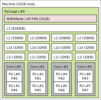
The compiler I’m using is clang v14.0. Benchmarking is done through Google Benchmark.For sanity, after each benchmark, I compare the result to PyTorch’s MMM implementation to make sure my implementation is correct.
| implementation | time (ms) |
|---|---|
| Naive Implementation (RCI) | 4481 |
| Naive Implementation (RCI) + compiler flags | 1621 |
| Naive Implementation (RCI) + flags + register accumulate | 1512 |
| Cache-aware loop reorder (RIC) | 89 |
| Loop reorder (RIC) + L1 tiling on I | 70 |
| Loop reorder (RIC) + L1 tiling on I + multithreading on R&C | 16 |
| Numpy (MKL) | 8 |
Naive implementation
Let’s start with a basic nested for-loop:
template <int rows, int columns, int inners>
inline void matmulImplNaive(const float *left, const float *right,
                            float *result) {
  for (int row = 0; row < rows; row++) {
    for (int col = 0; col < columns; col++) {
      for (int inner = 0; inner < inners; inner++) {
        result[row * columns + col] +=
            left[row * columns + inner] * right[inner * columns + col];
} } } }
We hard-code the matrix dimensions, by templating them. This makes it easier for the compiler to optimize, but makes the comparison against BLAS unfair since BLAS kernels have to work for all matrix sizes. In practice, a good BLAS library will have multiple implementations of matrix multiplication implemented for different size ranges. At runtime, based on the matrix dimensions, it’ll decide on which one to use. However, fixed matrix dimensions commonly appear in practice, for example when JIT-compiling a neural network where the batch size is known. Plus, the MKL implementation is so close to the theoretical maximum that it’ll serve as a good target.
Compiled with clang and default flags, this takes 4.4s.
The first, easy fix is to adjust the compiler flags.
First, we enable optimizations via -O3.
Then we tell the compiler to generate code that is specific to this microarchitecture (in our case Haswell) via -march=native.
This allows the compiler to output code that may not run on CPUs of a different microarchitecture, making it non-portable.
Lastly, we use -ffast-math allowing the compiler to do associative float math and promising it that there’ll be no NaNs / Infs in our program.Which may or may not be reasonable! See this post about the dangers of this innocent-sounding fastmath flag.
Combined these flags bring down runtime to 1.6s.
Another straightforward improvement is to perform the inner dot-product in a register, and only write out the result once the dot-product is finished.
template <int rows, int columns, int inners>
inline void matmulImplNaiveRegisterAcc(const float *left, const float *right,
                                       float *result) {
  for (int row = 0; row < rows; row++) {
    for (int col = 0; col < columns; col++) {
      float acc = 0.0;
      for (int inner = 0; inner < inners; inner++) {
        acc += left[row * columns + inner] * right[inner * columns + col];
      }
      result[row * columns + col] = acc;
} } }
This is a slight improvement, down to 1.5s. I tried figuring out if it was legal for the compiler to optimize away the inner store, but couldn’t get a definite answer. After inlining, the compiler could figure out where the pointers come from, and since they aren’t marked as volatile, get rid of some stores. In any case, it’s better to write the register accumulation ourselves by hand, instead of relying on the compiler.
Cache-aware implementation
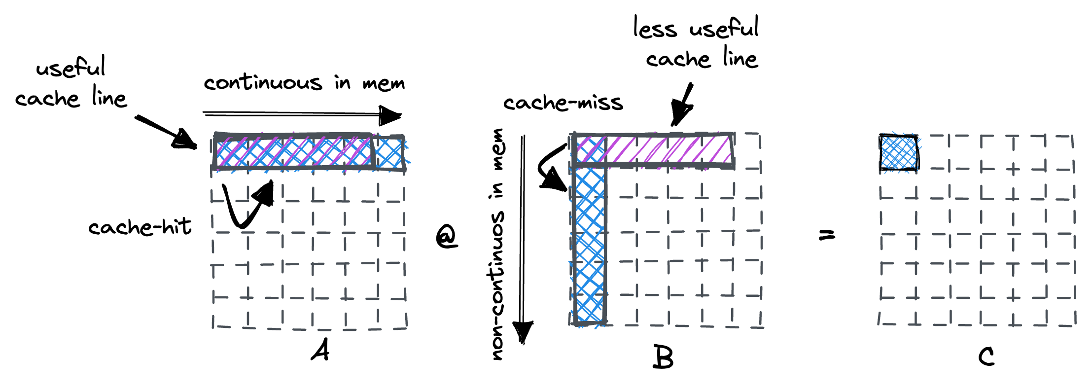
Multidimensional matrices are represented in memory using a strided representation.For a more detailed explanation, see this blogpost. In most programming languages you expect the matrix to be row-continuous, meaning that iterating through a single row by incrementing the column results in sequential memory access.

This makes it clear why the inner, most important loop of our matrix multiplication is very cache unfriendly. Normally, the processor loads data from memory using fixed-size cache lines, commonly 64 Byte large. When iterating over the row of A, we incur a cache miss on the first entry. The cache-line fetch by the processor will hold within it the next 15 floats as well, which is a good use of cache.
However, for matrix B, we walk down the rows, occurring a cache-miss at every step. At 1024 rows * 64 Byte cache lines, that means we’ve loaded a total of 64KB from memory once we reach the bottom row. On my specific CPU, the L1d cache is 32KB large, meaning later cache lines will kick earlier cache lines from the cache. Once we’ve reached the final row, the first rows of A & B are gone from the cache, and computing the next dot-product will start fetching all over again.
To fix this, we reorder the two inner-most loops:
template <int rows, int columns, int inners>
inline void matmulImplLoopOrder(const float *left, const float *right,
                                float *result) {
  for (int row = 0; row < rows; row++) {
    for (int inner = 0; inner < inners; inner++) {
      for (int col = 0; col < columns; col++) {
        result[row * columns + col] +=
            left[row * columns + inner] * right[inner * columns + col];
} } } }
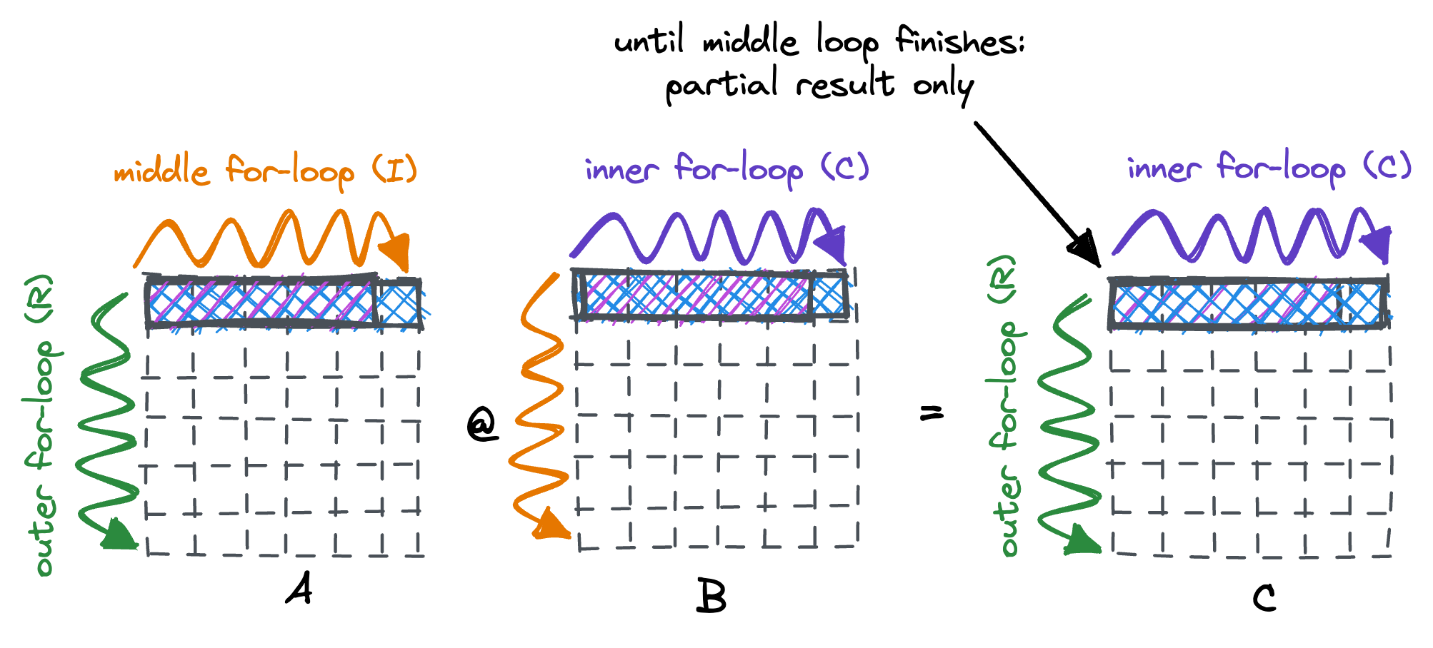
The improvement is quite spectacular, bringing runtime down to 89ms. A 16x improvement! Our inner loops now iterate through B & C in a memory sequential manner. The only time we do a large jump in memory access is when our middle loop finishes and we need to fetch the first row of B again. Since we’re now only computing a partial result in the inner loop, we cannot perform the accumulation in a single register anymore.
Looking at the compiled output on compiler explorer, the loop reordering also enabled vectorization.With the naive loop order the compiler was already using the VFMADD instruction, but only on a single fp32 at a time.
The relevant parts of the assembly look like this:
; In the loop setup, load a single fp32 from the current A row
; and broadcast it to all 8 entries of the ymm0 register
; vbroadcastss ymm0, dword ptr [rsi + 4*r8]

; In each instruction, load 8 entries from
; the current row of B into a ymm register
vmovups ymm1, ymmword ptr [rbx + 4*rbp - 96]
vmovups ymm2, ymmword ptr [rbx + 4*rbp - 64]
vmovups ymm3, ymmword ptr [rbx + 4*rbp - 32]
vmovups ymm4, ymmword ptr [rbx + 4*rbp]
; In each instruction, multipy the current entry of A (ymm0) times
; the entries of C (ymm1-4) and add partial results from C (memory load)
vfmadd213ps ymm1, ymm0, ymmword ptr [rcx + 4*rbp - 96] ; ymm1 = (ymm0 * ymm1) + mem
vfmadd213ps ymm2, ymm0, ymmword ptr [rcx + 4*rbp - 64] ; ymm2 = (ymm0 * ymm2) + mem
vfmadd213ps ymm3, ymm0, ymmword ptr [rcx + 4*rbp - 32] ; ymm3 = (ymm0 * ymm3) + mem
vfmadd213ps ymm4, ymm0, ymmword ptr [rcx + 4*rbp] ; ymm4 = (ymm0 * ymm4) + mem
; Store the partial results back to C's memory
vmovups ymmword ptr [rcx + 4*rbp - 96], ymm1
vmovups ymmword ptr [rcx + 4*rbp - 64], ymm2
vmovups ymmword ptr [rcx + 4*rbp - 32], ymm3
vmovups ymmword ptr [rcx + 4*rbp], ymm4
Tiling
We just saw how reordering our loops made the caches happy and brought a lot of performance. Next, we’ll cover a technique called tiling, sometimes also called cache blocking.
To motivate this: Assume this toy example of multiplying two 6x6 matrices and an L1d cache that fits 36 floats, is fully associativeThis means every cache line from main memory can be placed at any location into the cache. and has an omniscientThough a FIFO replacement policy should suffice in our case. cache replacement policy. When we reach the end of our middle for-loop (over the I-dimension), our cache is full and the first two rows of B have already been evicted. This means that upon starting the 2nd iteration of the outer for-loop and accessing B[I=0, C=0] we incur a cache miss. Similarly, due to the FIFO nature of our hypothetical L1d cache, none of the rows of B we access during our middle for-loop will be cached once we need them.
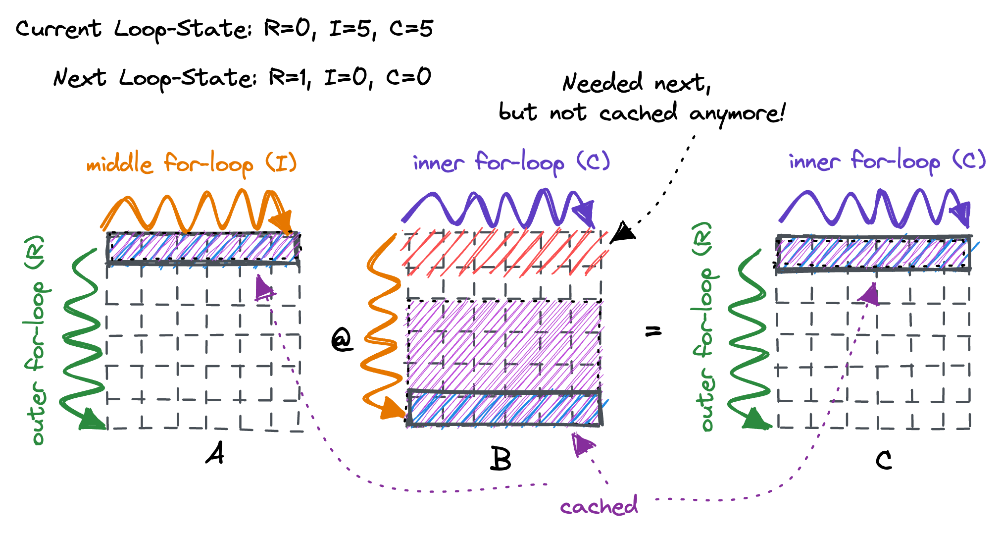
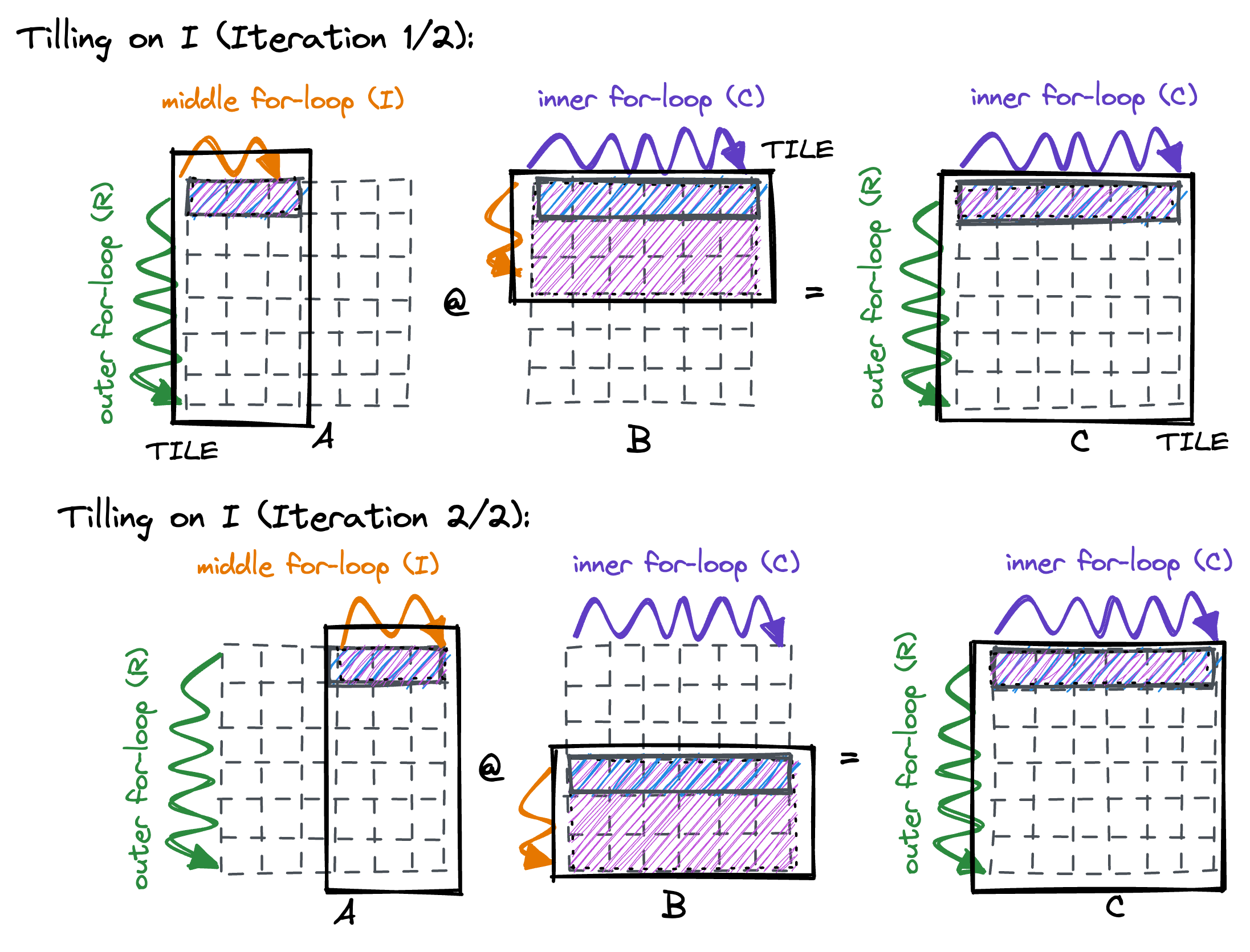
To solve this issue, we tile on the middle for-loop by introducing an additional outer loop with 2 iterations. By splitting the middle-loop in 2 parts, we ensure that we get no more cache misses in the middle loop, in all but the first iteration of the outer loop for each tile.
def matmulImplTiling(left, right, result) {
  # iteration 1
  for row in range(6):
    for inner in range(3):
      for column in range(6):
        result[row, column] += left[row, inner] * right[inner, column]

  # iteration 2
  for row in range(6):
    for inner in range(3, 6):
      for column in range(6):
        result[row, column] += left[row, inner] * right[inner, column]
A visualization might help make this clear. The block boxes are the tiles that we iterate over, the colored arrows denote our for-loop iterations. Displayed are both the first and second iterations of our new outer loop.
In Cpp, and implemented for arbitrary tile sizes, the code looks like this:
template <int rows, int columns, int inners, int tileSize>
inline void matmulImplTiling(const float *left, const float *right,
                             float *result) {
  for (int innerTile = 0; innerTile < inners; innerTile += tileSize) {
    for (int row = 0; row < rows; row++) {
      int innerTileEnd = std::min(inners, innerTile + tileSize);
      for (int inner = innerTile; inner < innerTileEnd; inner++) {
        for (int column = 0; column < columns; column++) {
          result[row * columns + column] +=
              left[row * inners + inner] * right[inner * columns + column];
} } } } }
In reality, picking the tile size is not that simple, since caches are seldomly fully associative. Further, operating system context switching (either to other userspace processes, or to interrupt routines) may pollute the cache in ways we cannot predict. In theory, the hot-set of our middle loop consists of:
- 1024 sliced rows of A: 1024 *
TILESIZE* 4B TILESIZErows of B:TILESIZE* 1024 * 4B- 1 row of C: 1024 * 4B
At an L1d cache size (per core) of 32KB, the optimal tile size is ~3.5. I grid searched through all reasonable values, and the optimal tile sizes ended up being significantly bigger. At a tile size of 16, the runtime went to 70ms. The optimal tile size will also be influenced by the loop overhead, and by how well the prefetcher can predict our memory accesses. Searching through many different combinations to find one that fits the microarchitecture well is common practice.For example, see the Atlas project.
Tiling on multiple dimensions
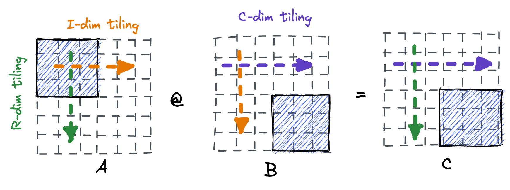
Similar to our tiling on the inner dimension, we can also perform tiling on the rows, and eventually on the columns. There are diminishing returns here for our small-sized matrices, but for larger matrices this makes sense. Each new dimension that we tile on allows us to make the working set of our inner loops smaller while introducing extra overhead.
Multithreaded matrix multiplication
As the last step, we’ll enable multithreading by using OpenMP.
To pick a good strategy it’s important to consider the dependencies of each entry in the result matrix C.
We want to avoid having to do partial summing between threads, which would either require atomics or locking.As a distant aside, the input dependencies show how recent deep learning Transformer models can partition the 2 linear layers that are part of their Transformer block across GPUs (Tensor parallelism) with only a single MPI communication step.  The first layer is column-partitioned on the weight matrix and produces column-partitioned output. The second layer is row-partitioned on the weight matrix, and its output is MPI.AllReduce’d (sum) into the final result.
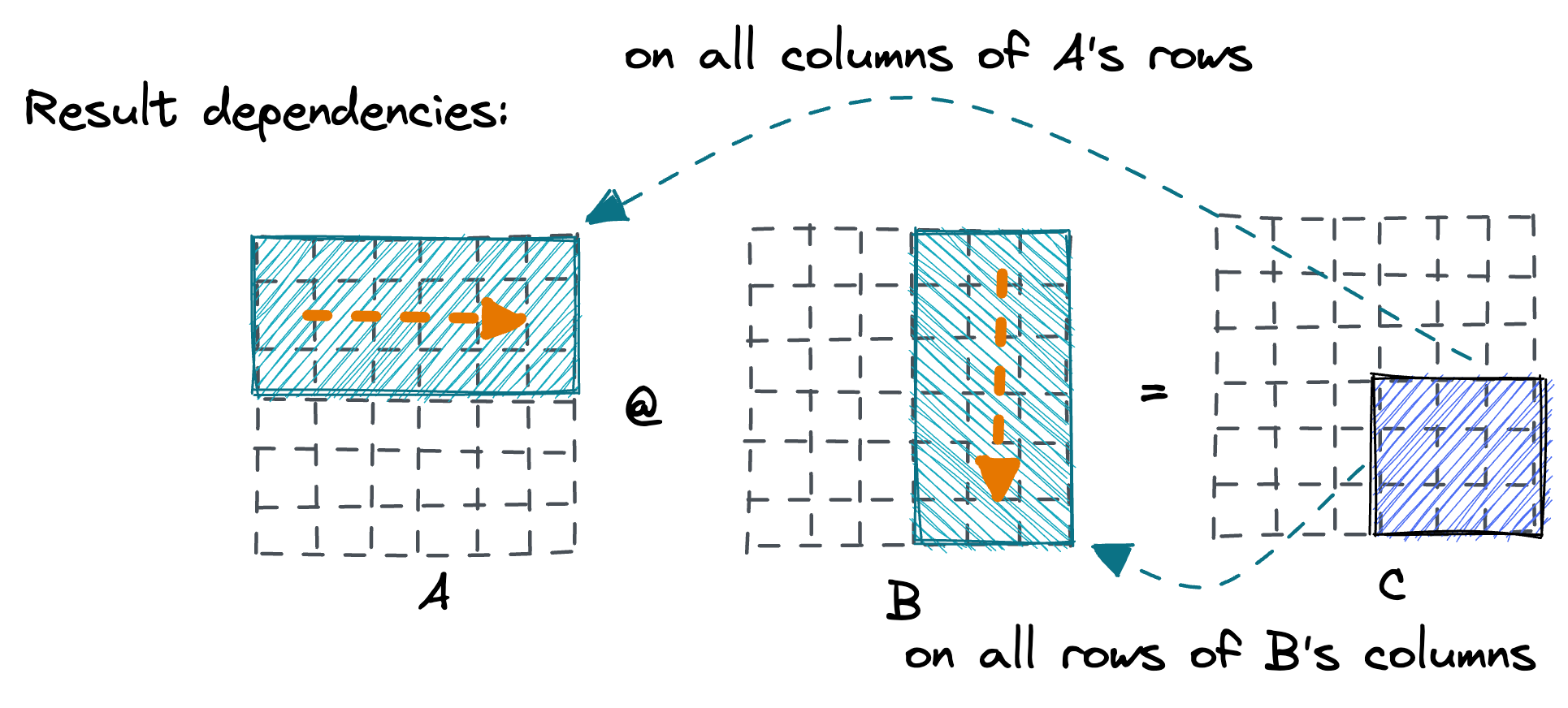
One way to divide the work among threads without the need to perform communication is by partitioning the rows and columns.Partitioning our toy 6x6 MMM between 4 threads: 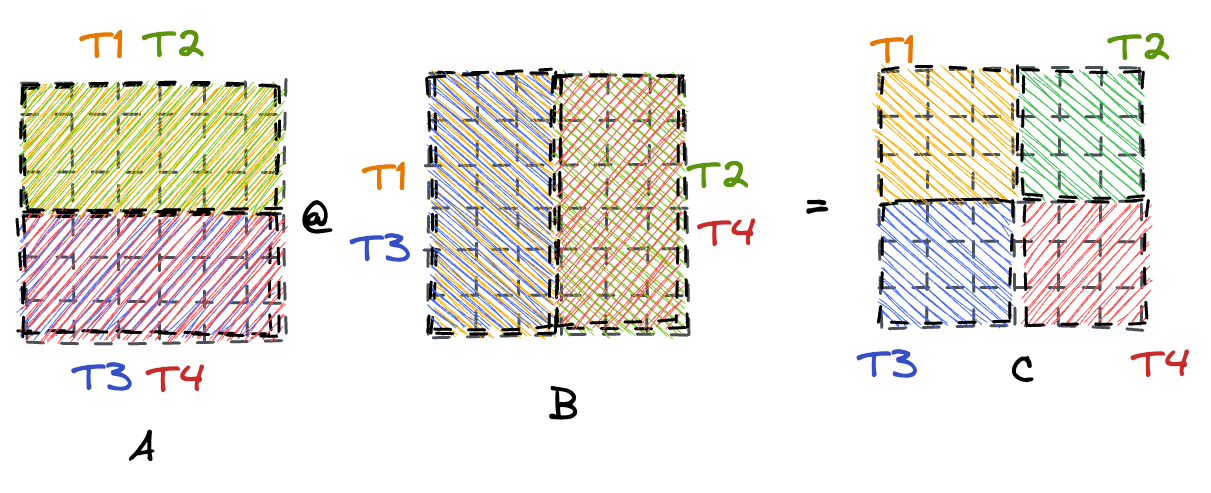 Each half of A & B needs to be read by two threads, but each thread computes its chunk of the output matrix C independently.
We split both the rows and columns into chunks of 4, giving us a total of 16 pieces of work, which we divide amongst 8 hyperthreads.
template <int rows, int columns, int inners,
          int tileSize = ROW_COL_PARALLEL_INNER_TILING_TILE_SIZE>
inline void matmulImplRowColParallelInnerTiling(const float *left,
                                                const float *right,
                                                float *result) {
#pragma omp parallel for shared(result, left, right) default(none) \
  collapse(2) num_threads(8)
  for (int rowTile = 0; rowTile < rows; rowTile += 256) {
    for (int columnTile = 0; columnTile < columns; columnTile += 256) {
      for (int innerTile = 0; innerTile < inners; innerTile += tileSize) {
        for (int row = rowTile; row < rowTile + 256; row++) {
          int innerTileEnd = std::min(inners, innerTile + tileSize);
          for (int inner = innerTile; inner < innerTileEnd; inner++) {
            for (int col = columnTile; col < columnTile + 256; col++) {
              result[row * columns + col] +=
                  left[row * inners + inner] * right[inner * columns + col];
} } } } } } }
The runtime of the final implementation is around 16ms.
Conclusion
Optimizing matrix multiplication is a fun exercise. It touches upon loop reordering, cache-aware programming and proper work distribution during multithreading. A BLAS implementation will probably also implement tiling for registers, and multi-dimensional tiling for all caches of the L1-L2-L3 hierarchy, among a few other optimizations that we didn’t cover here.
While writing this code it became apparent to me how easy it is to get lost while optimizing even a simple algorithm like matrix multiplication. You really need to have a strong mental model of the workings of your CPU, and a well-oiled benchmarking & testing setup to be able to iterate quickly.
Notes
- There are other algorithm’s for matrix multiplication that have an asymptotic runtime that’s faster than O(n^3), like the Coppersmith - Winograd algorithm that runs in O(n^2.3755). However, these algorithms have large constant factors, making them slower for all commonly encountered matrix sizes. To my knowledge, no BLAS library uses them.
- Just for comparison, a 2021 MacBook Pro with an M1 Pro chip runs the same Numpy code in 1ms, if you use Apple’s
accelerateBLAS implementation. The M1 chips have undocumented matrix-matrix assembly instructions that only Apple can compile for, which is where this speedup comes from (with OpenBLAS, the MBP takes ~8ms). Similar AMX instructions (but documented) are included in Intel’s Sapphire Rapids microarchitecture. - I was led down this rabbit hole of optimization when I stumbled over marek.ai/matrix-multiplication-on-cpu a few weeks ago.
- github.com/flame/how-to-optimize-gemm goes much further and explains how to actually reach BLAS-like performance from scratch.
