Data-Parallel Distributed Training of Deep Learning Models
September 2022
In this post, I want to have a look at a common technique for distributing model training: data parallelism.
It allows you to train your model faster by replicating the model among multiple compute nodes, and dividing the dataset among them.
Data parallelism works particularly well for models that are very parameter efficientMeaning a high ratio of FLOPS per forward pass / #parameters., like CNNs.
At the end of the post, we’ll look at some code for implementing data parallelism efficiently, taken from my tiny Python library ShallowSpeed.
Dependencies in Backpropagation and the Pebble-graph
Understanding data parallelism requires a good mental model of standard sequential backpropagation and the dependencies of each step.To learn more about backpropagation, I can recommend this digital book by Michael Nielson as well as Mathematics for Machine Learning. Both are available for free online. Personally, I’ve profited a lot from implementing backprop from scratch using just Numpy.
To simplify things, I’ll only be talking about sequential models, where output = LayerN(LayerN-1(...(Layer1(Input)))).
In the diagrams below, I’m illustrating the functional building blocks used for implementing backpropagation.
Each block takes inputs from the left and transforms them into outputs on the right.
The purpose of the Cache block is to store its input data until it’s next retrieved.

After having run backpropagation to compute the gradients, we use the optimizer to update the weights.

In general, any state we’re holding during the training process comes from:
- layer weights.
- cached layer outputs, also called activations.
- gradients with respect to (w.r.t.) weights, also just called gradients.
- gradients w.r.t. inputs, also called errors.The input gradients rarely show up in memory demand calculations, since we ‘backprop the error through the network’, meaning we operate inplace on the errors and only ever need to store one of them.
- optimizer state.Unless you’re using a stateless optimizer like stochastic gradient descent.
Putting the building blocks together, we end up with a full picture of how the cache is used during forward and backward passes. We call this the pebble graph of backpropagation. The pebble graph is great: if you understand it, it will be much easier to understand many concepts in distributed training.Originally, the concept of the pebble graph comes from this post about OpenAI’s implementation of gradient checkpointing.
The pebble graph below illustrates how the cached activations are built up during the forward pass and discarded once the corresponding backward pass is run. We see how the gradients w.r.t each layer’s weights are available (purple) after having run the backwards pass for a given layer.
Data-Parallel Training (DP)
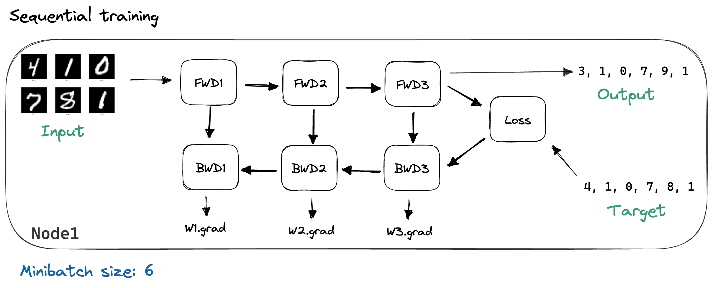
We described backpropagation above as it would be used in sequential training, where we have a single compute node, which has our model loaded in memory. During each iteration of training, we load the next minibatch and perform a forward pass through the model while caching each layer’s outputs. Then, we calculate the loss and run the backward pass, which calculates our gradients. This process is illustrated below, using MNIST images as our example input data.
Data parallelism works by duplicating the model across N machines. We split our minibatchThe naming here is not always consistent, and minibatches are often also just called batches. into N chunks and have each machine process one chunk.
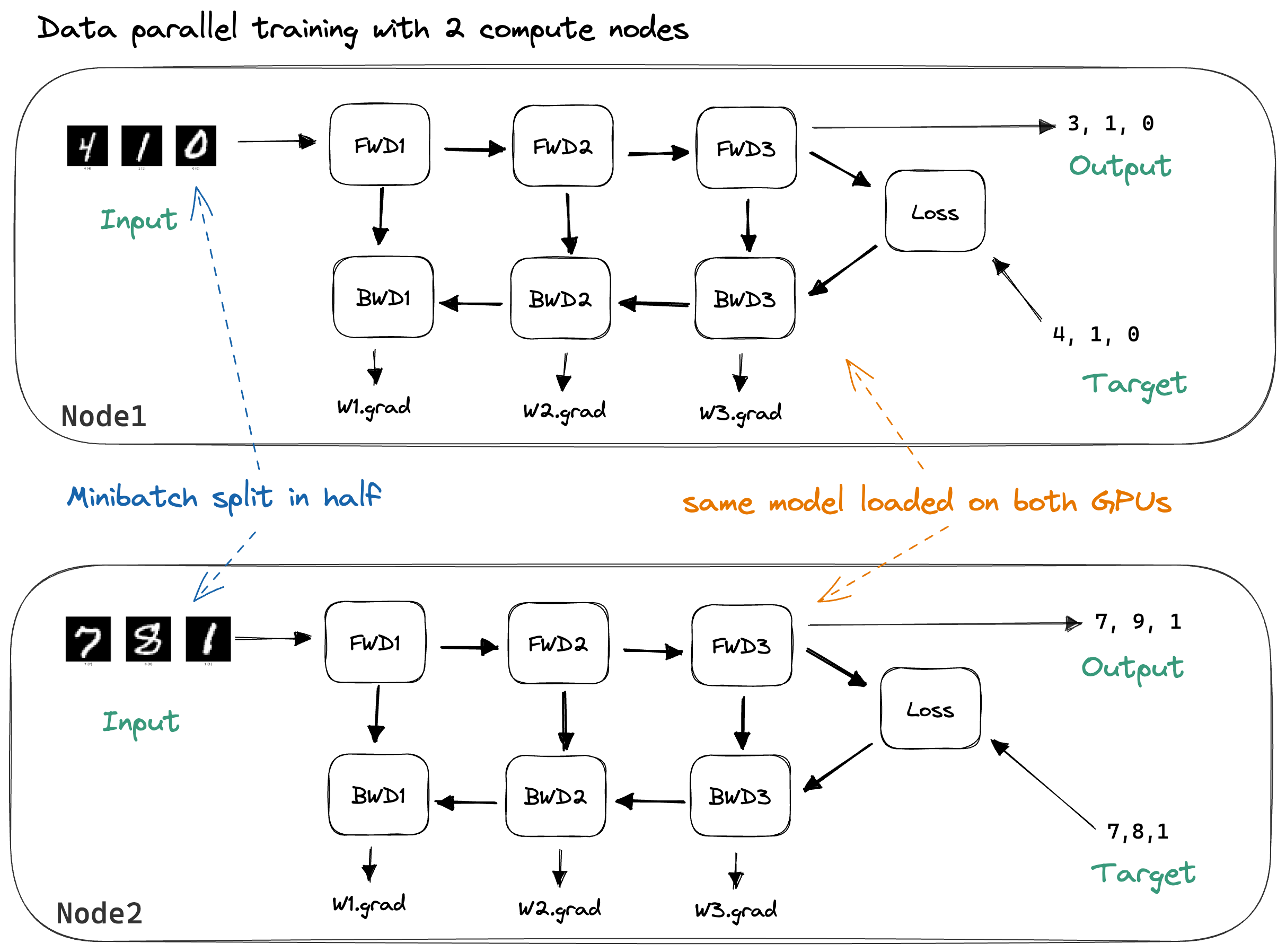
By splitting across multiple nodes, there’s less work to do for each node, and, if we neglect communication overhead, our training should be 2x faster. The samples in our batch can be independently processed,Notable exception: Batch norm. hence communication is not required during the forward pass (which calculates the output for each sample) nor during the backward pass (which calculates the gradient of a single sample’s loss w.r.t. the weights).
To achieve sequential consistencyI’ll call a distributed algorithm sequentially consistent if the resulting gradients are the same as if we had calculated them using sequential training on a single machine., we need to synchronize the gradients before updating our weights. The most commonly used loss functions are means over the loss of individual samples:
\[\text{loss(batch)}=\frac{1}{N}\sum_{i=0}^{\text{batchsize}}\text{loss}(\text{input}_{i}, \text{target}_i)\]Conveniently, the gradient of a sum is the sum of the gradients of each term. Hence, we can calculate the gradients of the samples independently on each machine and sum them up before performing the weight update.If you’re using stochastic gradient descent (SGD), there’s no difference between synchronizing the weights instead of the gradients, because \(\frac{1}{N} \sum_i \left(W + \lambda\nabla W_i\right) = W + \frac{\lambda}{N}\sum_i\nabla W_i\). However, this doesn’t work for stateful optimizers like Adam because updating the state is a non-linear function of the gradient. If we use Adam and sync the weights instead of the gradients, the optimizer states on each node diverge and we lose sequential consistency. After the synchronization, we want the gradients on each node to be the same:
\[\nabla W^{\text{sync'd}}= \frac{1}{\text{\#Nodes}}\sum_{i=0}^{\text{\#Nodes}}\nabla W_{i}^{\text{local}}\]Once the sync is complete we can perform the weight update and update our optimizer states.
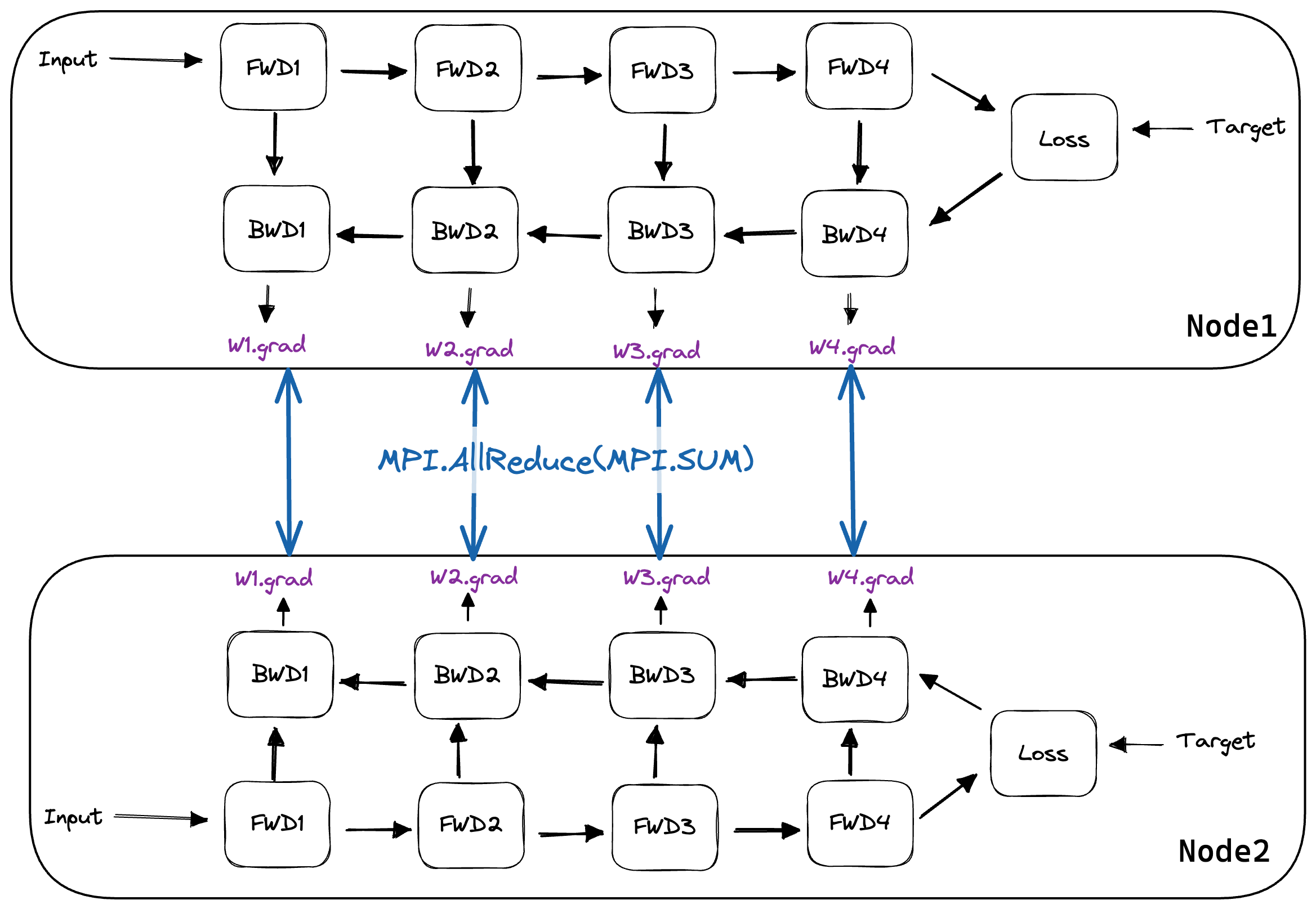
Summing up the distributed gradients and making the sum available on every node is achieved using the MPI.AllReduce operation.MPI stands for Message Passing Interface and is a specification (not an implementation) of multiple so-called ‘communication primitives’ that achieve common distributed communication tasks like distributing a block of data among all nodes, sending data from Node1 to Node2, collecting data from all nodes at Node0, etc. Here’s a link to my favorite MPI tutorial.
Mathematically, data-parallel training is sequentially consistent.
However, this doesn’t mean that we get equal outputs between sequential training and data parallel training in practice.
To add up the gradients, we need to use the MPI operation AllReduce, which collects the individual results from each node, computes the reduction from all of them (in our case, SUM of the gradients of the minibatches), and communicates the result back to all nodes.
AllReduce chooses the ordering for summing up the gradients for us, for example choosing (Node1 + Node2) + Node3 over Node1 + (Node2 + Node3).
This wouldn’t be a problem if this summation were commutative and associative.
Unfortunately, floating-point math is not associative,Wikipedia explaining the non-associativity, also here’s a link drop to my favourite visual explanation of the bit-level floating point representation. hence the result will not be exactly equal to sequential training.
In real-life systems, the difference between the expected gradients from sequential training versus gradients from data-parallel training is small enough that we can just ignore this issue.
However, it’s good to keep in mind that the gradients will not match, and debugging will be a little more difficult.
More Details on AllReduce in Data-Parallel Training
Let’s discuss AllReduce as used in data-parallel training a bit more.
I won’t talk about AllReduce itself too much, and instead point to two existing good blogposts on the implementation details of the AllReduce operator for DNN training, like this one about Baidu’s Ring-AllReduce and this one about Ring- and Tree-AllReduce.The MPI Spec guarantees that the result of AllReduce is exactly the same on each node. This is not straightforward, due to the non-associativity of floating-point math. Hence we have to make sure that local reductions happen in the same order. This naive algorithm for example would not fulfill the spec, since the local sums happen in different orders: 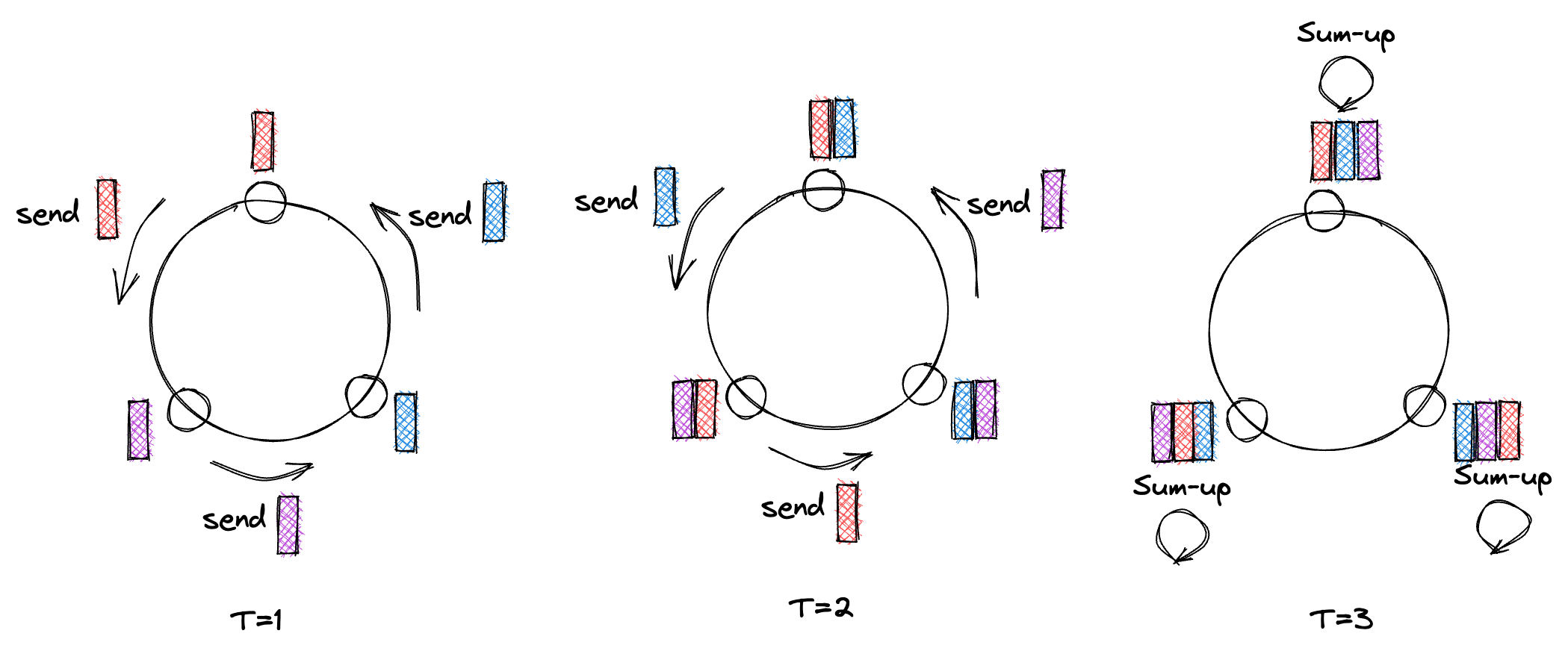 However, let’s briefly talk about the bandwidth and latency of a Ring AllReduce (one of the most common algorithms for implementing AllReduce).
- Bandwidth: Using a Ring AllReduce, each node needs to transfer \(2(\#nodes-1)\frac{\text{\#params}}{\text{\#nodes}}\) floats between itself and it’s two ring neighbours. Discarding the \(\frac{1}{\#nodes}\%\) inaccuracy, the size of data transferred doesn’t increase if we add more nodes. Further, Ring AllReduce is bandwidth optimal, meaning there is no way to achieve the same task but to transfer less data.This allows us to lower-bound the time spent on communication as \(\frac{\text{model size}}{\text{bandwidth}}\), assuming a full duplex connection, as during Ring AllReduce every node is sending & receiving at the same time.
- Latency: Again for Ring AllReduce, we need to perform #nodes-1 steps for
MPI.ReduceScatter, and #nodes-1 steps forMPI.AllGather. This means that while adding more nodes doesn’t require bigger data transfer, it does require linearly more communication rounds. How much that impacts the overall runtime will depend on the latency between your nodes.
We can visualize how AllReduce is used below. Here, once the gradients are calculated, AllReduce is performed using all nodes in our MPI.Communicator.
Integrating Data Parallelism into the Backwards Pass
Now we take a look at some of the code from ShallowSpeed to get a better grasp of the aforementioned concepts.
The straightforward way of implementing data-parallel distributed training is to run a full forward & backward pass, and before calling optimizer.step(), syncing the gradients.
In PyTorch, this would look like this:Because we’re blocking until the gradient AllReduce is done, we can perform the reduction in-place without using additional memory.
for param in model.parameters():
    comm.Allreduce(MPI.IN_PLACE, param.grad, op=MPI.SUM)
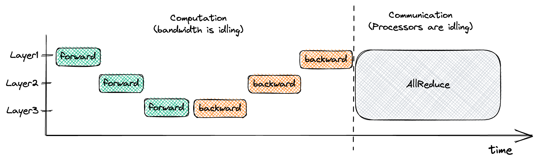
This is suboptimal since it divides our training into two stages. During the first stage (forward & backward pass) we’re waiting for the processors to finish computing, while our network is doing nothing. During the second stage (AllReduce) our network is communicating as fast as possible, while the processors are twiddling their fans.
We can visualize this type of training below:
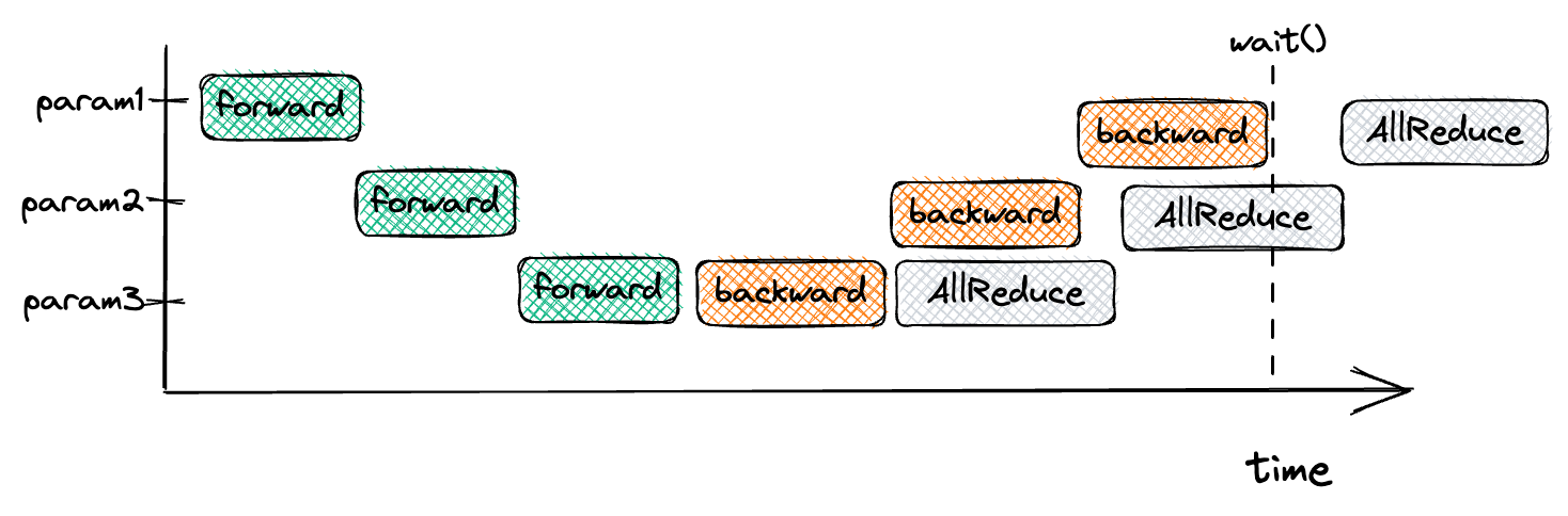
But notice that in the image above that, for example, the gradients of Layer3 are available once we’ve performed the backwards pass through Layer3. If we start a non-blocking AllReduce for Layer3’s parameters are soon as they are ready, our network will be busy doing useful work while our processors are independently calculating the gradients for Layer2. This strategy, called interleaving of communication and computation, allows us to optimize our training. We can visualize this interleaved implementation of data parallel training as so:
Normally, this is implemented through hooking into the Autograd systems:PyTorch doesn’t expose the hooks necessary to implement interleaved DP yourself. However, internally the DistributedDataParallel module is implemented as I describe it here.
def backprop_allreduce_gradient(comm, param):
    # we don't touch param.grad until the AllReduce is done, so we do it inplace
    param._request = comm.Iallreduce(
        sendbuf=MPI.IN_PLACE, recvbuf=param.grad, op=MPI.SUM
    )

autograd.register_grad_hook(backprop_allreduce_gradient)
The hook is triggered once a parameter’s gradient is ready:This introduces a lot of communication overhead, particularly if our parameters are small. Hence PyTorch’s DDP will collect gradients into buckets of a certain size, performing a single AllReduce for the whole bucket once all parameters in it have their gradients ready. Increasing the bucket size will lower communication overhead while potentially decreasing the amount of communication & computation interleaving.
def backward(self, dout):
    result = dout
    for layer in reversed(self.layers):
        result = layer.backward(result)
        for hook in self._grad_hooks:
            for param in layer.parameters():
                hook(param)
To ensure we’ve finished all AllReduce operations before updating our weights, we block until all communication is done:
def wait_for_comms(params):
    requests = [param._request for param in params]
    MPI.Request.Waitall(requests)
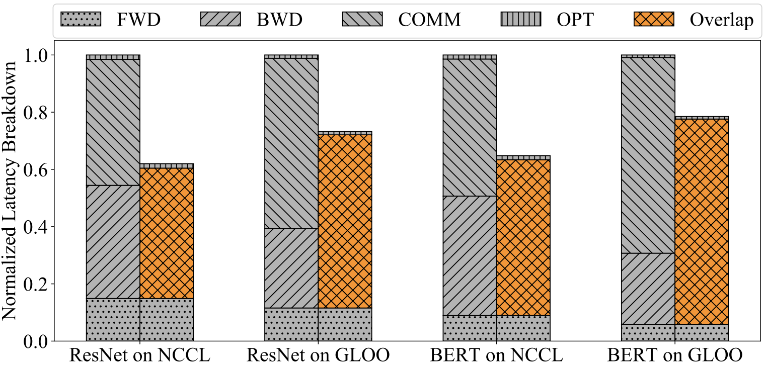
In the paper on PyTorch’s DistributedDataParallel module, they show that interleaving brings pretty big performance gains. The graph below shows a comparison of the runtime between non-interleaved distributed data-parallel training and interleaved training of two models using two different implementations of AllReduce: NCCL and GLOO. The forward passes for each ResNet and BERT take the same amount of time independent of the AllReduce implementation, they just normalized the y-axis.
Conclusion and Summary
So that was a quick introduction to data parallelism, which is a common way of speeding up training deep learning models if multiple compute nodes are available. It works particularly well if your network is parameter efficient since each batch requires sending all model weights over the networkData parallelism is often described as an all-or-nothing operation, but in theory it’d be possible to do data-parallel training on parts of your network (eg the most compute-expensive early CNN layers) while running the rest of the network sequentially on a different node. and if your batchsize is large. The batchsize is an upper limit on the degree of DP parallelism.Allowing a bigger batch size is the main motivation for using learning rate schedulers like LARS and LAMB. Small batches sizes mean small inputs, which decreases the operational intensity of matrix multiplication and that will lead to inefficient computation.
To get a better understanding of data parallelism, check out the PyTorch DDP paper, which details the implementation of data parallelism in PyTorch (as well as many more optimizations) and my ShallowSpeed library. ShallowSpeed implements data parallelism as described here from scratch. I tried to make the code as readable as possible, feel free to play around with it.
In part 2, I cover pipeline parallelism, which allows training models that do not fit into a single compute node’s memory.
Appendix
Memory Demand of DNN Training
Here I’m considering bfloat16 mixed-precision trainingMixed-precision training refers to performing the forward and backward pass at a lower precision (normally fp16 or bfloat16). This saves memory (the cached activations are smaller), and bandwidth (we need to transfer half the amount of data into the processor). Increasingly there is also hardware support for fast fp16/bfloat16 math, eg in Nvidia’s Tensor Cores, or x86 AMX instructions. For more info, see Mixed Precision Training (arXiv). using the Adam optimizer. The memory demand consists of the model state, the optimizer state, plus the activation state. For each parameter, we need to store its model + optimizer state. The activation state consists of the activations cached during the forward pass.
1.Model state:
- Parameter: fp32 source + bfloat16 replicaTechnically it wouldn’t be necessary to keep two replicas of the parameters around at different precisions. This is because for a fp32 value, loading only the first 2 bytes is equal to its representation in bfloat16.
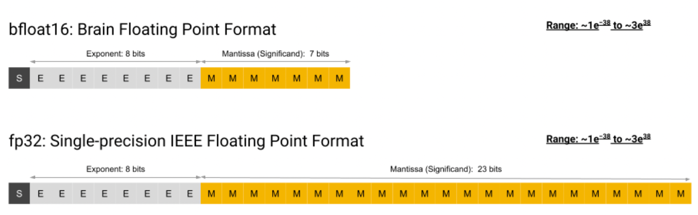 I assume most libraries use the bfloat16 replica because strided memory access on the float32 tensor would result in poor cache usage.
 - Its gradient: bfloat16Communicating only 2B per parameter halves the bandwidth necessary for the data-parallel gradient AllReduce.
2.Adam optimizer state:
- Momentum: fp32
- Variance: fp32
3.Activation state:
The activation state consists of whatever tensors we need to cache between the forward and the backward passes. For an MLP, we can estimate this as:There may be additional memory demand, depending on the activation function. For a backward pass through a ReLU, we can theoretically utilize the cached inputs of the next layer to compute the gradient, so we don’t need to cache anything extra.
We store the activations at 16-bit precision.
In total: We need to store 16 bytes for each model parameter for the model and optimizer state. To this, we add our cached activations, whose size depends on the particular model architecture.Note that the size of the cached activations increases linearly with the batch size. The storage requirement for the activations can be lessened by so-called gradient checkpointing, where only parts of the activations are cached, while others are re-computed as required.
A Bandwidth Optimization for Data-Parallel Training
Every implementation of data parallelism that I’ve looked at while writing this post synced the gradients using an AllReduce. However, a different sync strategy would be possible for the weight matrices.
The gradient w.r.t. W is computed as the outer product of the gradient coming from the next layer and the cached input. Illustrating this operation and the operand sizes:
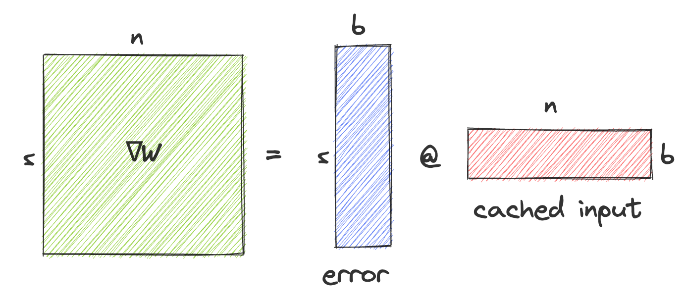
Instead of performing an AllReduce on \(\nabla W\) we could perform an AllGather on the error and on the cached activations, and then materialize \(\nabla W\) by performing the outer product on each node. For a square W, this would reduce the data transferred by each node from \(n^2\) to \(2nb\) where b is the batch size, and would therefore save bandwidth if \(b<\frac{1}{2}n\).
The downside would be increased code complexity and \(O(b*n^2)\) extra computation steps per node.