Pipeline-Parallelism: Distributed Training via Model Partitioning
October 2022
Pipeline parallelism makes it possible to train large models that don’t fit into a single GPU’s memory.Example: Huggingface’s BLOOM model is a 175B parameter Transformer model. Storing the weights as bfloat16 requires 350GB, but the GPUs they used to train BLOOM ‘only’ have 80GB of memory, and training requires much more memory than just loading the model weights. So their final training was distributed across 384 GPUs. This is made possible by assigning different layers of the model to different GPUs, a process called model partitioning. Implemented naively, model partitioning results in low GPU utilization. In this post, we’ll first discuss the naive implementation of pipeline parallelism and some of its problems. Then, we’ll talk about GPipe and PipeDream, two more recent algorithms that alleviate some of the issues with naive pipeline parallelism.
This is the second part of my series on distributed training of large-scale deep learning models. The first part, which covers data-parallel training, can be found here.
Naive Model Parallelism
Naive model parallelism is the most straightforward way of implementing pipeline-parallel training. We split our model into multiple parts, and assign each one to a GPU. Then we run regular training on minibatches, inserting communication steps at the boundaries where we’ve split the model.
Let’s take this 4-layer sequential model as an example:
\[\text{output}=\text{L}_4(\text{L}_3(\text{L}_2(\text{L}_1(\text{input}))))\]We split the computation among two GPUs as follows:
- GPU1 computes: \(\text{intermediate}=\text{L}_2(\text{L}_1(\text{input}))\)
- GPU2 computes: \(\text{output}=\text{L}_4(\text{L}_3(\text{intermediate}))\)
To complete a forward pass, we compute itermediate on GPU1 and transfer the resulting tensor to GPU2.
GPU2 then computes the output of the model and starts the backward pass.
For the backward pass, we send the gradients w.r.t. intermediate from GPU2 to GPU1.
GPU1 then completes the backward pass based on the gradients it was sent.
This way, the model parallel training results in the same outputs and gradients as single-node training.
Because the sending doesn’t modify any bits, naive model-parallel training is, unlike data-parallel training, bit-equal to sequential training. This makes debugging much easier.
The pebble graphIf you’re having difficulties understanding the pebble graph, the post on data parallelism introduced them more thoroughly. below illustrates naive model parallelism.
GPU1 performs its forward pass and caches the activations (red).
Then it uses MPI to send the outputs of L2 to the next GPU, GPU2.
GPU2 finishes the forward pass, calculates the loss using the target values, and starts the backward pass.
Once GPU2 is finished, the gradient w.r.t. L2’s output is sent to GPU1, which completes the backward pass.
Notice how we only use node-to-node communication (MPI.Send and MPI.Recv) and don’t need any collective communication primitives (so no MPI.AllReduce, as in data parallelism).
By looking at the pebble graph, we can observe some inefficiencies of naive model parallelism.
- Low GPU utilization: At any given time, only one GPU is busy, while the other GPU is idle. If we added more GPUs, each one would be busy only \(\frac{1}{\text{\#GPUs}}\)% of the time (neglecting communication overhead). Low utilization suggests that there may be a way to speed up training by assigning useful work to GPUs that are currently idling.
- No interleaving of communication and computation: While we’re sending intermediate outputs (FWD) and gradients (BWD) over the network, no GPU is doing anything. We already saw how interleaving computation and communication brings big benefits when we discussed data-parallelism.
- High memory demand: GPU1 holds all activations for the whole minibatch cached until the very end. If the batch size is large, this can create memory problems. Later we’ll talk about combining data and pipeline parallelism to solve this problem, but there are other ways to lessen the memory demand as well.
Let’s now look at ways to mitigate the inefficiencies of naive model parallelism. First up is the GPipe algorithm, which attains much higher GPU utilization compared to the naive model parallel algorithm.
The GPipe Algorithm: Splitting Minibatches into Microbatches
GPipe increases efficiency by splitting each minibatch into even smaller, equal-sized microbatches. We can then compute the forward and backward pass independently for each microbatch.As long as there is no batch norm. It’s possible to use batchnorm and GPipe by computing the normalizing statistics over the microbatch, which often works but isn’t equal to sequential training anymore. If we sum up the gradients for each microbatch, we get back the gradient over the whole batch.Because, just like for data parallel training, the gradient of a sum is the sum of the gradients of each term. This process is called gradient accumulation. As each layer exists only on one GPU, the summing-up of microbatch-gradients can be performed locally, without any communication.The local gradient accumulation is equal to sequential training mathematically speaking. Due to the non-associativity of floating-point math, the output will not be bit-equal though. However, this is seldom a problem in practice.
Let’s consider a model partitioned across 4 GPUs.The general problem of partitioning an arbitrary model among GPUs such that computation is balanced and communication is minimized is fairly difficult, and requires performance profiling. For Transformers is easy to solve since it consists of so-called ‘Transformer blocks’ that all have the same operations and dimensions. For naive pipeline parallelism, the resulting schedule would look like this:
| Timestep | 0 | 1 | 2 | 3 | 4 | 5 | 6 | 7 |
|---|---|---|---|---|---|---|---|---|
| GPU3 | FWD | BWD | ||||||
| GPU2 | FWD | BWD | ||||||
| GPU1 | FWD | BWD | ||||||
| GPU0 | FWD | BWD |
As mentioned previously, at any given point in time, only one GPU is busy. Further, each of these timesteps would take fairly long, since the GPU has to run the forward-pass for the whole minibatch.
With GPipe we now split our minibatch into microbatches, let’s say 4 of them.
| Timestep | 0 | 1 | 2 | 3 | 4 | 5 | 6 | 7 | 8 | 9 | 10 | 11 | 12 | 13 |
|---|---|---|---|---|---|---|---|---|---|---|---|---|---|---|
| GPU3 | F1 | F2 | F3 | F4 | B4 | B3 | B2 | B1 | ||||||
| GPU2 | F1 | F2 | F3 | F4 | B4 | B3 | B2 | B1 | ||||||
| GPU1 | F1 | F2 | F3 | F4 | B4 | B3 | B2 | B1 | ||||||
| GPU0 | F1 | F2 | F3 | F4 | B4 | B3 | B2 | B1 |
Here F1 means performing the forward pass of microbatch1 using the layer partition stored on the current GPU.
Importantly, each timestep in the GPipe schedule will be shorter than each timestep in the naive model parallel schedule, since with GPipe a GPU only works on a quarter of the minibatch at a time.However, splitting the minibatch into smaller microbatches will add overhead, partly because we need to launch more kernels in total. If the layers are small and the microbatches are small, there may not be enough opportunity for within-GPU parallelism to result in high CUDA core utilization.
Overall, GPipe and its microbatches are a big improvement over naive pipeline parallelism since now more than one GPU is doing useful work at the same time. Let’s look at some of the remaining inefficiencies of GPipe and how to might address them: The interleaving of comms and compute, pipeline bubbles, and memory demand.
GPipe: Interleaving of Computation and Communication
Unfortunately, there is not a lot of opportunity to interleave comms and compute if the forward and backward passes take the same amount of time for each GPU. This can be seen in the above table since each GPU cannot start processing a given microbatch before the previous GPU has finished processing that same microbatch. If all stages take the same amount of time, then we’ll still get distinct times of communication and computation.
The paper that originally introduced GPipe doesn’t cover this, but one option could be to split each minibatch in half. Then we could interleave communication of the first half with computation of the second half. Whether or not this makes sense in practice will depend on kernel and network timings.
Here’s a sketch of an interleaved version of GPipe:

The arrows show the dependencies for the first half of the first microbatch.
Let’s move on to the main inefficiency of GPipe, the size of the pipeline bubble.
GPipe: Pipeline Bubbles
Bubbles are spots in the pipeline where no useful work is being done.
They are caused by dependencies between the operations.
For example, GPU4 cannot execute F1 until GPU3 has executed F1 and transmitted the result.

The fraction of time wasted on the bubble depends on the pipeline-depth n and the number of microbatches m:To explain the terms in the formula: The \(2mn\) term is the overall amount of useful work, and stems from each of the \(n\) nodes performing \(m\) forward and \(m\) backward passes. \(2n(m + n - 1)\) is the overall time for a single batch. During each the forward and backward pass, each node performs \(m\) items of work and waits \(n-1\) timesteps for new work to arrive.
So increasing the size of the minibatches, which increases the number of microbatches m, is necessary for making the bubble fraction small.Some example calculations for a batch consisting of a single microbatch vs 4 microbatches: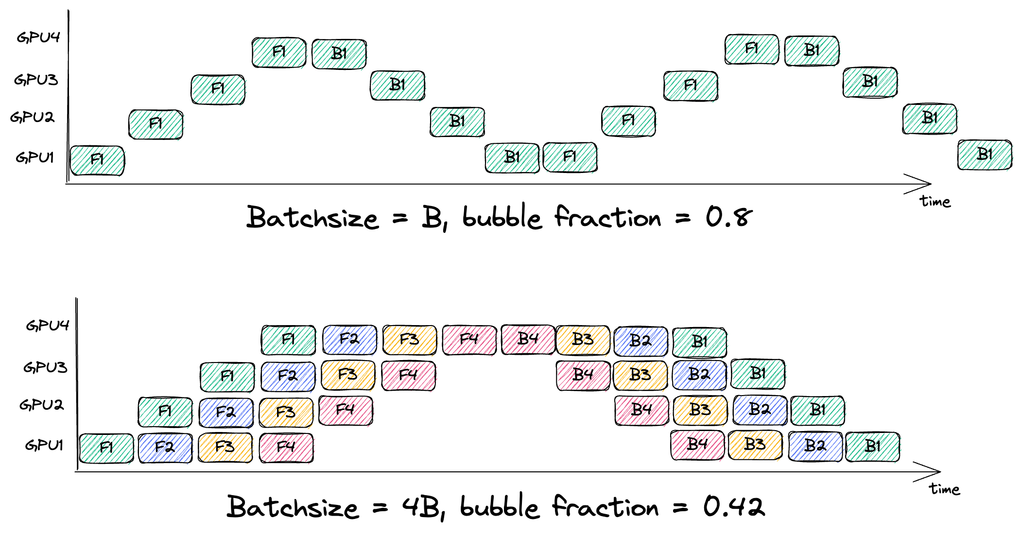 Large minibatch sizes require careful learning rate scalingSee learning rate schedulers like LARS and LAMB. and will increase the memory demand for caching the activations, which we’ll get to next.
GPipe: Memory demand
Increasing the batch size increases the memory demand for cached activations linearly.For a more detailed analysis of memory demand of NN training, see the appendix of my post on data parallelism.
In GPipe, we need to cache the activations for each microbatch from the time it was forward‘ed until the corresponding backward.
To take GPU0 as an example, looking at the table above, the activations for microbatch1 are held in memory from timestep 0 until timestep 13.
In the GPipe paper, the authors utilize gradient checkpointingSee also the original paper on gradient checkpointing, as well as this excellent blogpost. to bring down the memory demand. In gradient checkpointing, instead of caching all activations necessary to compute our gradients, we recompute the activations on the fly during the backward pass. This lowers the memory demand but increases our computational costs.
Let’s assume all layers have roughly the same size. The memory demand for caching the activations amounts to
\[O(\text{batchsize} \cdot \frac{\text{\#total layers}}{\text{\#GPUs}})\]for each GPU.To explain the formula: For each layer, we need to cache its inputs. Assuming the layer-width is a constant, a single cached input is of size \(O(\text{batchsize})\). Instead, we could perform gradient checkpointing and only cache the inputs on the layer boundaries (i.e. cache the tensor that has been sent to us from the previous GPU). This lowers the peak memory demand on each GPU to
\[O(\text{batchsize} + \frac{\text{\#total layers}}{\text{\#GPUs}}\frac{\text{batchsize}}{\text{\#microbatches}})\]Why? \(O(\text{batchsize})\) is the space necessary for caching the boundary activation. When performing the backward pass for a given microbatch, we need to re-materialize the activations that are necessary for computing the gradients for that microbatch. This requires \(O(\frac{\text{batchsize}}{\text{\#microbatches}})\) space for each of the \(O(\frac{\text{\#total layers}}{\text{\#GPUs}})\) layers on each GPU. The following plot visualizes the memory demand of GPipe with gradient checkpointing. It shows two GPUs during the backward pass. GPU3 has recomputed the activations for microbatch 3, while GPU4 has recomputed activations for microbatch 2. At the GPU boundary, the activations for the whole batch stay cached from the forward until the backward pass.

Next, I’ll cover PipeDream, a different algorithm for pipeline parallel training. PipeDream offers us another option for decreasing the memory demand of microbatch training, which is orthogonal to gradient checkpointing.
The PipeDream Algorithm: Interleaving Forwards- and Backwards-Passes for Different microbatches
PipeDream starts the backward pass for a microbatch as soon as the final pipeline stage has completed the corresponding forward pass. We can discard the cached activation for the m’th microbatch as soon as we perform the corresponding backward pass. With PipeDream, this backward pass happens earlier than in GPipe, which lessens the memory demand.
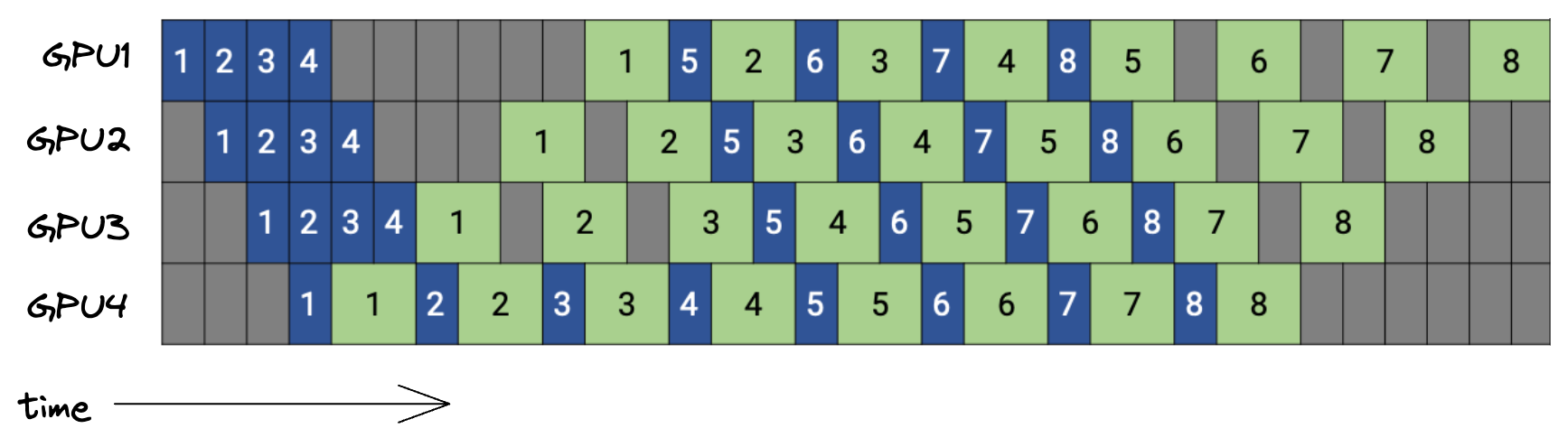
Below is a plot of the PipeDream schedule, with 4 GPUs and 8 microbatches.Figure taken from the Megatron LM paper. Strictly speaking, this schedule is called PipeDream Flush 1F1B, which I’ll explain later. Blue boxes are forward passes, numbered with their microbatch id, while the backward passes are in green.
Let’s think about memory demand for a second. For both GPipe and PipeDream, the memory demand for caching activations can be formalized as (w/o gradient checkpointing)
\[O(\text{\#max microbatches in flight}\cdot \text{microbatch-size} \cdot \frac{\text{\#total layers}}{\text{\#GPUs}})\]With the above PipeDream schedule, we have at most as many microbatches in flightA microbatch is in-flight if we performed >1 forward pass for it, but haven’t completed all the backward passes yet. as the pipeline is deep.The pipeline depth is the total number of GPUs that process a microbatch until all gradients for that microbatch have been computed. This becomes obvious when looking at GPU1 in the above plot. During the steady state, GPU1 forward’s a new microbatch only after completing a backward pass. The steady state is the time of peak memory usage, and happens after the so-called warmup phase: 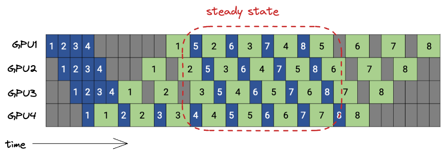 Contrast this with GPipe, where all microbatches are in flight at some point during the schedule, resulting in a higher memory demand for caching activations.
Using the above example, with PipeDream we’d have a maximum of 4 microbatches in flight, while with GPipe it’d be 8 microbatches,As we have 8 microbatches per batch in this example, GPipe will first compute the FWD pass for all microbatches before starting the first BWD pass. Look at the above GPipe table for reference, but keep in mind that the table assumes 4 microbatches per batch. doubling the memory demand for cached activations.
Contrast this with GPipe, where all microbatches are in flight at some point during the schedule, resulting in a higher memory demand for caching activations.
Using the above example, with PipeDream we’d have a maximum of 4 microbatches in flight, while with GPipe it’d be 8 microbatches,As we have 8 microbatches per batch in this example, GPipe will first compute the FWD pass for all microbatches before starting the first BWD pass. Look at the above GPipe table for reference, but keep in mind that the table assumes 4 microbatches per batch. doubling the memory demand for cached activations.
In terms of bubble fraction, there is no difference between PipeDream and GPipe. The bubble is a result of the inherent dependencies between the operations before on the microbatches, which PipeDream doesn’t change.Visually, looking at the above PipeDream plot if you shift the blue forward passes left and the green backward passes right, you get GPipe. This explains why the bubble fraction is the same.
There are a lot of variations of the PipeDream schedule, and I cannot say that I’ve grokked all of them.
The above schedule is called 1F1B because during the steady state each node is alternating between performing a forward and a backward pass.
Notice how the above schedule is still sequentially consistent.
In the original PipeDream paper as well as in the Megatron LM paper there are many more variations. By avoiding the pipeline flushFlushing a pipeline means not scheduling any new operations until all currently scheduled operations are done processing. Once the pipeline is flushed, we know that our gradients (accumulated over the microbatches) are sequentially consistent. Then we perform the optimizer step. at the end of processing each batch, one can increase efficiency by decreasing the bubble fraction. However, this means the algorithm isn’t sequentially consistent anymore, which may hurt convergence speed. A slower convergence will force you to train for longer, so non-sequentially consistent PipeDream schedules may not actually be useful for lessening training time and cost. I’m not sure how widely used the non-sequentially consistent versions of PipeDream are as a result.
Let’s briefly look at the volume of networked communication that’s necessary for implementing pipeline parallelism. This analysis is the same for GPipe and PipeDream.
Pipeline parallelism: Communication Volume
For simplicity, let’s assume a model with only dense layers, which all have equal dimension N. During the forward pass, each GPU will send and receive data of size \(\text{batchsize} \cdot N\). The same holds for the backwards pass, bringing our total communication volume to \((\text{\#GPUs} - 1) \cdot 2\cdot\text{batchsize} \cdot N\) floats.The -1 terms comes from the initial GPU not having to receive and the last GPU not having to send anything.
Compare this to data parallelism, where each GPU has to AllReduce the gradients for all its layers. In our dense model example, using Ring AllReduce, each GPU needs to transfer roughly \(2 \cdot \frac{\text{\#layers} \cdot N^2}{\text{\#GPUs}}\) floats. Depending on the configuration of your model and training setup, data parallelism may be more communication intensive. However, as we saw we can interleave the data parallel communication quite well, which isn’t possible with pipeline parallelism.
So far, we have looked at three ways of implementing pipeline parallelism: naive model parallelism, GPipe, and PipeDream. Next, I’ll show how pipeline parallelism can be combined with data parallelism, allowing one to use even bigger batchsizes without running out of memory.
Combining Data and Pipeline Parallelism
Data and pipeline parallelism are orthogonal and can both be used at the same time, as long as the batchsize is big enough to result in a sensible microbatchsize.
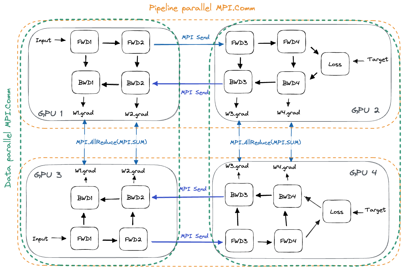
- For pipeline parallelism, each GPU needs to communicate with the next pipeline stage (during FWD) as well as with the previous pipeline stage (during BWD).
- For data parallelism, each GPU needs to communicate with all other GPUs that are assigned the same model layers. We need to AllReduce the gradients among all layer replicas after the pipeline has been flushed.We can interleave the AllReduce with the backward pass of the final microbatch to reduce training time, just as in regular data parallel training.
In practice, the orthogonal communication partners for pipeline and data parallelism are implemented using MPI Communicators. These form subgroups of all GPUs and allow performing collective communication only within the subgroup. Any given GPU-X will be part of two communicators, one containing all GPUs that hold the same layer slice as GPU-X (data parallelism), and one containing the GPUs that hold the other layer slices of GPU-X’s model replica (pipeline parallelism). See the below plot for an illustration:
Combining different degrees of data and pipeline parallelism for a given pool of GPUs requires a modular software architecture, which I’ll cover next.
Pipeline Parallelism: Implementation of GPipe
The below code snippets are taken from my implementation of data and pipeline parallelism in my ShallowSpeed library.
Contrary to data parallelism, pipeline parallelism requires no collective communication and therefore no explicit synchronization between workers. Microsoft’s DeepSpeed library uses a software design where each GPU contains a single worker, that processes instructions as given by the schedule. The DeepSpeed worker model is attractive since the schedules are static. This means each worker’s schedule is computed when the worker is started, and then executed repeatedly for each minibatch, requiring no communication about scheduling among the workers during training. PyTorch’s Pipeline design is quite different, using queues for communicating among the workers, where workers forward tasks to each other.
For the GPipe implementation in my ShallowSpeed library, I followed the worker model.
Before starting the processing of a minibatch, we first zero out the current gradients. Once the minibatch is done processing, we update the weights through an optimizer step.
def minibatch_steps(self):
    yield [ZeroGrad()]

    # STAGE 1: First, we FWD all microbatches
    for microbatch_id in range(self.num_micro_batches):
        yield self.steps_FWD_microbatch(microbatch_id)

    # at this position, all microbatches are in flight and
    # memory demand is highest

    # STAGE 2: Then, we BWD all microbatches
    for microbatch_id in reversed(range(self.num_micro_batches)):
        yield from self.steps_BWD_microbatch(microbatch_id)

    # updating the weights is the last step of processing any batch
    yield [OptimizerStep()]
The steps of the schedule are implemented as a Python generator.
Let’s look at the steps necessary for forward-ing a microbatch:
def steps_FWD_microbatch(self, microbatch_id):
    cmds = []
    if self.is_first_stage:
        # first pipeline stage loads data from disk
        cmds.append(LoadMicroBatchInput(microbatch_id=microbatch_id))
    else:
        # all other stages receive activations from prev pipeline stage
        cmds.append(RecvActivations())

    cmds.append(Forward(microbatch_id=microbatch_id))

    if not self.is_last_stage:
        # all but the last pipeline stage send their output to next stage
        cmds.append(SendActivations())
    return cmds
We pass the microbatch id to all operations that need to store into the activation cache. This is because, for some microbatch-X, we need to be able to retrieve the activations cached during microbatch-X FWD during the microbatch-X BWD pass.
Finally, let’s look at the steps of the backward pass for a single microbatch:
def steps_BWD_microbatch(self, microbatch_id):
    cmds = []
    if self.is_last_stage:
        # last pipeline stage loads data from disk
        cmds.append(LoadMicroBatchTarget(microbatch_id=microbatch_id))
    else:
        # all other stages wait to receive grad from prev stage
        cmds.append(RecvOutputGrad())

    # the first microBatch is the lasted one that goes through backward pass
    if self.is_first_microbatch(microbatch_id):
        # interleaved backprop and AllReduce during last microBatch of BWD
        cmds.append(BackwardGradAllReduce(microbatch_id=microbatch_id))
    else:
        cmds.append(BackwardGradAcc(microbatch_id=microbatch_id))

    if not self.is_first_stage:
        # all but last pipeline stage send their input grad to prev stage
        cmds.append(SendInputGrad())
    yield cmds
Conclusion and Summary
That concludes the introduction to pipeline parallelism. Pipeline parallelism is a way of training large models that do not fit into a single GPU’s memory, by partitioning the model’s layers across GPUs. We perform GPU-to-GPU communication between the model partitions during the forward pass (to send activations) and the backward pass (to send gradients). We saw how naive model parallelism suffers from poor GPU utilization. This is alleviated by GPipe, which splits minibatches into smaller microbatches, keeping multiple GPUs busy at any given time. We saw how PipeDream, another algorithm for pipeline parallelism, achieves a smaller memory footprint than GPipe by starting backward passes earlier. Pipeline parallelism can be combined with data parallelism to further decrease the memory demand for each worker.
To get a better understanding of pipeline parallelism, check out the GPipe and PipeDream papers. The PipeDream paper also explains their profiling strategy for fairly partitioning arbitrary models among GPUs. This Megatron-LM is another great read. It talks about combining data parallelism, PipeDream, and tensor parallelism efficiently while also preserving sequential consistency.
I implemented GPipe-parallel training on CPU from scratch for ShallowSpeed. I tried to make the code as readable as possible, feel free to play around with it.
Further links
- Lilian Weng’s post about training models on many GPUs.
- Huggingface’s post about the tech behind BLOOM training.
Appendix
General Hardware Setting
It’s important to keep in mind the hardware systems that these models are trained on. Normal GPU clusters used for training consist of multiple compute nodes that are connected using either fast ethernet or a specialized communication backend like InfiniBand. Each compute node will contain multiple GPUs. The GPUs communicate with the CPU and CPU RAM via PCIe. The GPUs within a single compute node are commonly connected via a fast interconnect like Nvidia’s NVLink.
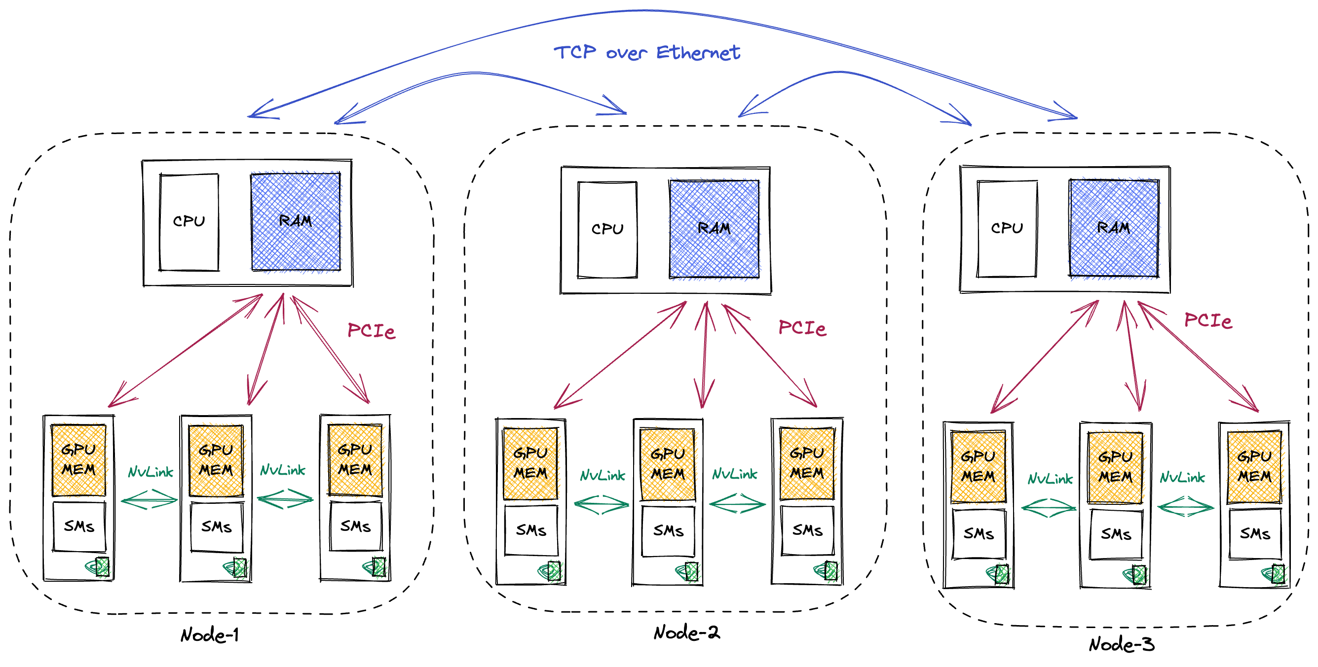
This hierarchy is important to keep in mind when evaluating different training distribution schemes since GPUs within the same compute node can communicate much faster than GPUs located on different nodes.As a concrete example, BLOOM was trained on 48 compute nodes, with 8 GPUs each (source). Rough estimates for the bandwidth at each level (these are all a bit optimistic, real bandwidth will be lower rather than higher):These are just rough numbers, rounded so that they’re easier to memorize. What matters is the order-of-magnitude, as the actual value will depend strongly on the cluster setup. For reference, look at the Wikipedia for NVLink and InfiniBand.
- NVLink (GPU to GPU): ~450GB/s up and down, making for a total 900GB/s of bandwidth.
- PCIe (GPU Mem to CPU RAM): ~25GB/s up and down (for a 16x PCIe 4.0 connection).
- Ethernet (Node to Node, within same datacenter): ~10GB/s. The alternative is InfiniBand, which is faster at ~50GB/s. For NVLink and PCIe, the bandwidth scales linearly with the number of lanes connected.
Distributed Training Glossary
- Strong scalingVisual comparison of strong vs weak scaling:
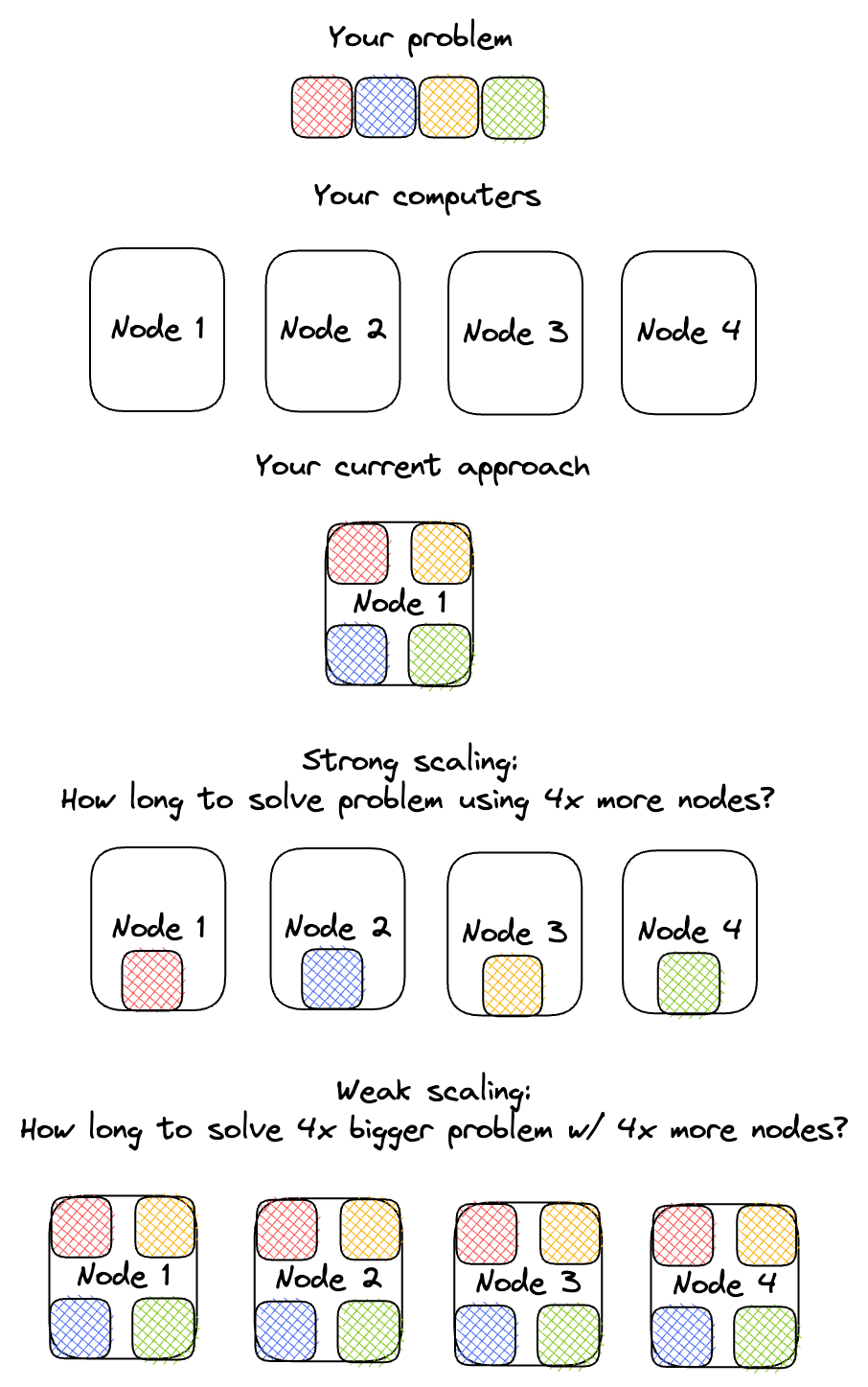 answers the question of how fast the training time decreases if we add more GPUs, while keeping the model size constant. Example: If you’re wondering how fast you could train your ResNet50 if you had 10 GPUs instead of 1, then you care about strong scaling.
 - Weak scaling answers the question of how long training takes if we add more GPUs while keeping the model size per GPU constant. Example: You suspect your model is performing poorly because it is too small, but your GPU’s memory is completely full. Weak scaling characteristics will tell you how much longer it will take to train a model of twice the size on 2 GPUs.
- I’ll call a distributed algorithm sequentially consistent if the resulting gradients are the same as if we had calculated them using sequential training on a single machine.As I mentioned in my post on data parallelism, sequential consistency doesn’t mean the results will be equal in practice, due to non-associativity of floating point math.
- Statistical efficiency determines how much some distributed training algorithm impacts the final accuracy of your model. If the algorithm is sequentially consistent, it will have perfect statistical efficiency.
- Algorithmic efficiency determines how much computation / memory / time some distributed algorithm will consume.These are super vague definitions, but I still think they’re useful for classifying the different pipeline parallel algorithms.